library(tidymodels)
library(tidyverse)Appendix D — Technical details
Once you start to develop models for larger datasets, you will realize that tuning models can take a long time. There are a few strategies to help speed up the process.
Work with smaller datasets during development of your workflow until you get your R code right. Then switch to the full dataset. Chapter 12 shows how to create a representative subset of your data. This is a good strategy if you are working with a large dataset and you are not sure if your code is correct.
Use parallel processing to speed up the tuning process. Approaches like cross-validation greatly benefit from this. Section D.1 shows how to do this. We made use of this approach in various chapters in this book. This is a good strategy that is useful for larger datasets.
Use caching to speed up the tuning process. Section D.2 shows how to use caching to speed up the tuning process. This is a good strategy for when you are confident in your code and results, and you work on describing and discussing them in the text.
Load required packages:
D.1 Parallel processing
Modern computers no longer exist of a single CPU, but have multiple cores. You can use these cores to speed up the tuning process. R has a variety of packages to setup and use parallel processing on your computer. The package future is one of them. At the start of your R or _Rmarkdown file, you need to setup the parallel processing environment.
library(future)
plan(multisession,
  workers = parallel::detectCores(logical = FALSE))
After importing the future package, we create a cluster of workers. The number of workers is set to the number of cores on your computer. You can change this number to a lower number if you want to keep some cores available for other tasks or if your calculations runs out of memory (RAM).
file <- "https://gedeck.github.io/DS-6030/datasets/UniversalBank.csv.gz"
data <- read_csv(file) %>%
  select(-c(ID, `ZIP Code`)) %>%
  rename(
    Personal.Loan = `Personal Loan`,
    Securities.Account = `Securities Account`,
    CD.Account = `CD Account`
  ) %>%
  mutate(
    Personal.Loan = factor(Personal.Loan, labels = c("Yes", "No"),
      levels = c(1, 0)),
    Education = factor(Education,
      labels = c("Undergrad", "Graduate", "Advanced")),
  )

formula <- Personal.Loan ~ Income + Family + CCAvg + Education +
  Mortgage + Securities.Account + CD.Account + Online + CreditCard
recipe_rf <- recipe(formula, data = data)
model_rf <- rand_forest(mode = "classification",
  mtry = tune(), trees = tune()) %>%
  set_engine("ranger")
workflow_rf <- workflow() %>%
  add_recipe(recipe_rf) %>%
  add_model(model_rf)
parameters <- extract_parameter_set_dials(workflow_rf)
parameters <- parameters %>%
  update(
    mtry = mtry(c(2, 6)),
    trees = trees(c(100, 500))
)set.seed(1)
# repeat 10-fold cross-validation five times
resamples <- vfold_cv(data, v = 10, repeats = 5)
timings <- tibble()
for (number_cores in 1:20) {
with(plan(multisession, workers = number_cores), {
# train random forest model five times using cross-validation
# and measure execution time
start_time <- Sys.time()
tune_rf <- tune_grid(
workflow_rf,
resamples = resamples,
grid = grid_regular(parameters, levels = c(5, 2))
)
end_time <- Sys.time()
time_taken <- round(end_time - start_time, 2)
if (length(timings) == 0) {
timings <- tibble(
number_cores = number_cores,
time_taken = time_taken
)
} else {
timings <- timings %>%
add_row(
number_cores = number_cores,
time_taken = time_taken
)
}
})
}
timings$average_time_taken <- as.numeric(timings$time_taken) / 5
timings$ideal <- timings$average_time_taken[1] / timings$number_coresWe train \(10 \times 5 \times 10 = 500\) models (10 tuning, 5 repeats, 10-fold cross-validation). Figure D.1 shows the reduction in tuning time when parallel processing is used.
ggplot(timings, aes(x = number_cores, y = average_time_taken)) +
  geom_line() +
  geom_line(aes(y = ideal), color = "grey") +
  geom_point() +
  geom_vline(
    xintercept = parallel::detectCores(logical = FALSE),
    color = "red") +
  xlab("Number of cores") +
  ylab("Average time required for tuning (seconds)")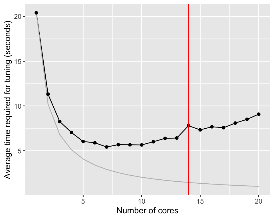
Without parallelization, tuning the random forest model takes about 20.4 seconds. Distributing the calculation on two cores, reduces the time to 11.3 seconds. If parallelization would be perfect, the time should be reduced to 10.2 seconds. There is overhead involved in parallelization and we can already see the effect of this here. Nevertheless, increasing the number of cores even more, brings the calculation time down to 5.4.
The improvement go through a minimum between 5 and 10 cores. After that, the average time required for tuning increases again slightly. The computer used for the graph was a M3 Macbook Pro with 14 cores.
On some computers, you might see hyperthreading. This is a technique to make the computer appear to have more cores than it actually has. This can be useful for tasks that require a lot of communication with other resources. However, for calculations like this, hyperthreading is not as efficient as physical cores.
TipUseful to know
When you use parallelization and you get error messages like this, your computer is running out of memory (RAM).
Error in unserialize(socklist[[n]]):
    error reading from connection
Error in serialize(data, node$con):
    error writing to connection
Error in `summary.connection()`: ! invalid connection
In this case, reduce the number of cores in the cluster. For example, set plan(multisession, workers = 4) to use only 4 cores.
NoteFurther information
The tidymodels package will already use parallelization if the a cluster is setup. However, if you want to parallelize your own code, you can use the foreach package. It’s fairly easy to use. See the following links for examples: - https://cran.r-project.org/web/packages/doParallel/vignettes/gettingstartedParallel.pdf gives a short overview on how to use the doParallel package. - https://www.blasbenito.com/post/02_parallelizing_loops_with_r/ is a more in depth introduction into parallelization with the foreach package.
D.2 Caching
Running the code in the previous chapter takes more than 156 seconds. Executing the code every time this document needs to be recreated, will make working with the document insufferable. We can use caching to speed up the process. Caching is a technique to save the results of a calculation and reuse them later. The next time the code is executed, the results are loaded from the cache instead of being recalculated.
Using caching with Rmarkdown is straightforward. Above we used the cache option in the code chunk header to enable caching. Here is the markup for the code chunk that loads and prepares the data.
```{r cache-prepare-model}
#| message: FALSE
#| warning: FALSE
#| cache: TRUE

code to load and prepare the model

```
Note two points here. Firstly, the code chunk has a name. Secondly, the code chunk header contains the cache: TRUE option. The name identifies the cache. If you change the code inside the code chunk, the cache is invalidated and the code is executed again. If you don’t specify a name, Rmarkdown will create a random name for the code chunk. This is not recommended as it can lead to issues later on.
We also use caching the code chunk that tunes the model.
```{r cache-time-tuning}
#| message: FALSE
#| warning: FALSE
#| cache: TRUE

code to tune the model

```
Like before, we use the cache: TRUE option which will cache the results of this code chunk too. Consider now the case where you knitted the document and both code chunks are cached and you make a change to the first code chunk which leads to a change of the data. When you knit the document again, this data are reloaded and preprocessed. The code chunk that tunes the model however was not changed and would in principle not be executed again. This would lead to invalid results. To avoid this, we use the dependson option in the code chunk header of the code chunk that tunes the model. The dependson option tells Rmarkdown that the code chunk that tunes the model depends on the code chunk that loads and prepares the model. If the code chunk that loads and prepares the model is executed, the code chunk that tunes the model will be executed too.
If you have a code chunk that depends on multiple previous code chunks, you can use a comma separated list of names in the dependson option. In this example, test3 depends on test1 and test2.
```{r test1}
#| cache: TRUE
x = 10
x
```

```{r test2}
#| cache: TRUE
#| dependson: test1
y = 2
y
```

```{r test3}
#| cache: TRUE
#| dependson: test1, test2
x + y
```
You can make a code chunk depend on all previous code chunks by using the dependson=knitr::all_labels() option.
TipUseful to know
Another option is to add the following code at the start of your document.
```{r}
knitr::opts_chunk$set(cache=TRUE, autodep=TRUE)
```
This will cache all code chunks in the document and automatically create the dependencies based on the variables used in and between code chunks.
If you use this approach together with parallelization, explicitly set the code that starts the cluster to not being cached.
```{r}
#| cache: FALSE
library(future)
plan(multisession,
    workers = parallel::detectCores(logical = FALSE))
```
NoteFurther information
- https://tune.tidymodels.org/articles/extras/optimizations.html more information on how to speed up your tidymodels code in particular with parallel processing.
- Caching has a lot more options that are not covered here. Check these sources for more information: