26 Threshold selection

In this example, we will

load and preprocess data
define a workflow
use cross-validation to determine a threshold using the F-statistic
train the final model
evaluate the model using cross-validation and holdout data
predict

using the Loan prediction dataset to illustrate the whole process.

Load the required packages:

library(tidyverse)
library(tidymodels)

Load and preprocess the data:

file <- "https://gedeck.github.io/DS-6030/datasets/loan_prediction.csv"
data <- read_csv(file, show_col_types = FALSE) %>%
  drop_na() %>%
  mutate(
    Gender = as.factor(Gender),
    Married = as.factor(Married),
    Dependents = gsub("\\+", "", Dependents) %>% as.numeric(),
    Education = as.factor(Education),
    Self_Employed = as.factor(Self_Employed),
    Credit_History = as.factor(Credit_History),
    Property_Area = as.factor(Property_Area),
    Loan_Status = factor(Loan_Status, levels = c("N", "Y"),
      labels = c("No", "Yes"))
  ) %>%
  select(-Loan_ID)

Split dataset into training and holdout data, prepare for cross-validation:

set.seed(123)
data_split <- initial_split(data, prop = 0.8, strata = Loan_Status)
train_data <- training(data_split)
holdout_data <- testing(data_split)

resamples <- vfold_cv(train_data, v = 10, strata = Loan_Status)
cv_metrics <- metric_set(roc_auc, accuracy)
cv_control <- control_resamples(save_pred = TRUE)

Define the recipe, the model specification (elasticnet logistic regression), and combine them into a workflow:

formula <- Loan_Status ~ Gender + Married + Dependents + Education +
  Self_Employed + ApplicantIncome + CoapplicantIncome + LoanAmount +
  Loan_Amount_Term + Credit_History + Property_Area
recipe_spec <- recipe(formula, data = train_data) %>%
  step_dummy(all_nominal(), -all_outcomes())

model_spec <- logistic_reg(engine = "glm", mode = "classification")

wf <- workflow() %>%
  add_model(model_spec) %>%
  add_recipe(recipe_spec)

Use the workflow for cross-validation and training the final model using the full dataset:

result_cv <-  fit_resamples(wf, resamples, metrics = cv_metrics,
  control = cv_control)
fitted_model <- wf %>% fit(train_data)

Estimate model performance using the cross-validation results and the holdout data:

cv_results <- collect_metrics(result_cv) %>%
  select(.metric, mean) %>%
  rename(.estimate = mean) %>%
  mutate(result = "Cross-validation", threshold = 0.5)
holdout_predictions <- augment(fitted_model, new_data = holdout_data)
holdout_results <-  bind_rows(
  c(roc_auc(holdout_predictions, Loan_Status, .pred_Yes,
      event_level = "second")),
  c(accuracy(holdout_predictions, Loan_Status, .pred_class))) %>%
  select(-.estimator) %>%
  mutate(result = "Holdout", threshold = 0.5)

performance <- probably::threshold_perf(
  result_cv %>% collect_predictions(),
  Loan_Status, .pred_Yes, seq(0.1, 0.9, 0.01), event_level = "second",
  metrics = metric_set(j_index, f_meas, kap))

max_values <- performance %>%
  arrange(desc(.threshold)) %>%
  group_by(.metric) %>%
  filter(.estimate == max(.estimate)) %>%
  filter(row_number() == 1)
ggplot(performance, aes(x = .threshold, y = .estimate, color = .metric)) +
  geom_line() +
  geom_vline(data = max_values, aes(xintercept = .threshold, color = .metric))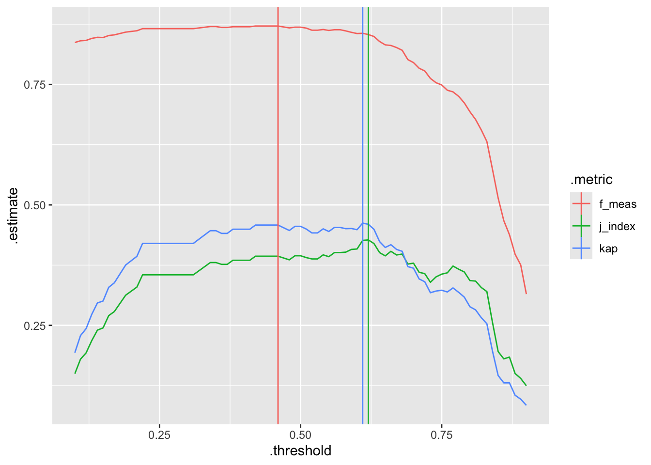

Figure 26.1: Performance metrics as a function of the classification threshold.

We decide to select the threshold that maximizes the F-measure:

threshold <- max_values %>%
  filter(.metric == "f_meas") %>%
  pull(.threshold)

We can now calculate the performance metrics using predictions at the selected threshold.

cv_predictions <- collect_predictions(result_cv) %>%
  mutate(
    .pred_class = factor(ifelse(.pred_Yes >= threshold, "Yes", "No"))
  )
cv_threshold_results <-  bind_rows(
  c(accuracy(cv_predictions, Loan_Status, .pred_class))
) %>%
  select(-.estimator) %>%
  mutate(result = "Cross-validation", threshold = threshold)
holdout_predictions <- augment(fitted_model, new_data = holdout_data) %>%
  mutate(
    .pred_class = factor(ifelse(.pred_Yes >= threshold, "Yes", "No"))
  )
holdout_threshold_results <-  bind_rows(
  c(accuracy(holdout_predictions, Loan_Status, .pred_class))
) %>%
  select(-.estimator) %>%
  mutate(result = "Holdout", threshold = threshold)

The performance metrics are summarized in the following table.

bind_rows(
  cv_results,
  holdout_results,
  cv_threshold_results,
  holdout_threshold_results,
) %>%
  pivot_wider(names_from = .metric, values_from = .estimate) %>%
  kableExtra::kbl(caption = "Model performance metrics", digits = 3) %>%
  kableExtra::kable_styling(full_width = FALSE)

result	threshold	accuracy	roc_auc
Cross-validation	0.50	0.799	0.752
Holdout	0.50	0.825	0.733
Cross-validation	0.46	0.802	NA
Holdout	0.46	0.835	NA

Model performance metrics

We can see that the reduced threshold leads to a higher accuracy.

Code

The code of this chapter is summarized here.

Show the code

knitr::opts_chunk$set(echo = TRUE, cache = TRUE, autodep = TRUE,
  fig.align = "center")
library(tidyverse)
library(tidymodels)
file <- "https://gedeck.github.io/DS-6030/datasets/loan_prediction.csv"
data <- read_csv(file, show_col_types = FALSE) %>%
  drop_na() %>%
  mutate(
    Gender = as.factor(Gender),
    Married = as.factor(Married),
    Dependents = gsub("\\+", "", Dependents) %>% as.numeric(),
    Education = as.factor(Education),
    Self_Employed = as.factor(Self_Employed),
    Credit_History = as.factor(Credit_History),
    Property_Area = as.factor(Property_Area),
    Loan_Status = factor(Loan_Status, levels = c("N", "Y"),
      labels = c("No", "Yes"))
  ) %>%
  select(-Loan_ID)
set.seed(123)
data_split <- initial_split(data, prop = 0.8, strata = Loan_Status)
train_data <- training(data_split)
holdout_data <- testing(data_split)

resamples <- vfold_cv(train_data, v = 10, strata = Loan_Status)
cv_metrics <- metric_set(roc_auc, accuracy)
cv_control <- control_resamples(save_pred = TRUE)
formula <- Loan_Status ~ Gender + Married + Dependents + Education +
  Self_Employed + ApplicantIncome + CoapplicantIncome + LoanAmount +
  Loan_Amount_Term + Credit_History + Property_Area
recipe_spec <- recipe(formula, data = train_data) %>%
  step_dummy(all_nominal(), -all_outcomes())

model_spec <- logistic_reg(engine = "glm", mode = "classification")

wf <- workflow() %>%
  add_model(model_spec) %>%
  add_recipe(recipe_spec)
result_cv <-  fit_resamples(wf, resamples, metrics = cv_metrics,
  control = cv_control)
fitted_model <- wf %>% fit(train_data)
cv_results <- collect_metrics(result_cv) %>%
  select(.metric, mean) %>%
  rename(.estimate = mean) %>%
  mutate(result = "Cross-validation", threshold = 0.5)
holdout_predictions <- augment(fitted_model, new_data = holdout_data)
holdout_results <-  bind_rows(
  c(roc_auc(holdout_predictions, Loan_Status, .pred_Yes,
      event_level = "second")),
  c(accuracy(holdout_predictions, Loan_Status, .pred_class))) %>%
  select(-.estimator) %>%
  mutate(result = "Holdout", threshold = 0.5)
performance <- probably::threshold_perf(
  result_cv %>% collect_predictions(),
  Loan_Status, .pred_Yes, seq(0.1, 0.9, 0.01), event_level = "second",
  metrics = metric_set(j_index, f_meas, kap))
max_values <- performance %>%
  arrange(desc(.threshold)) %>%
  group_by(.metric) %>%
  filter(.estimate == max(.estimate)) %>%
  filter(row_number() == 1)
ggplot(performance, aes(x = .threshold, y = .estimate, color = .metric)) +
  geom_line() +
  geom_vline(data = max_values, aes(xintercept = .threshold, color = .metric))
threshold <- max_values %>%
  filter(.metric == "f_meas") %>%
  pull(.threshold)
cv_predictions <- collect_predictions(result_cv) %>%
  mutate(
    .pred_class = factor(ifelse(.pred_Yes >= threshold, "Yes", "No"))
  )
cv_threshold_results <-  bind_rows(
  c(accuracy(cv_predictions, Loan_Status, .pred_class))
) %>%
  select(-.estimator) %>%
  mutate(result = "Cross-validation", threshold = threshold)
holdout_predictions <- augment(fitted_model, new_data = holdout_data) %>%
  mutate(
    .pred_class = factor(ifelse(.pred_Yes >= threshold, "Yes", "No"))
  )
holdout_threshold_results <-  bind_rows(
  c(accuracy(holdout_predictions, Loan_Status, .pred_class))
) %>%
  select(-.estimator) %>%
  mutate(result = "Holdout", threshold = threshold)
bind_rows(
  cv_results,
  holdout_results,
  cv_threshold_results,
  holdout_threshold_results,
) %>%
  pivot_wider(names_from = .metric, values_from = .estimate) %>%
  kableExtra::kbl(caption = "Model performance metrics", digits = 3) %>%
  kableExtra::kable_styling(full_width = FALSE)