library(tidyverse)
library(tidymodels)10 Training classification models using tidymodels
Regression models predict a quantitative, continuous numerical outcome. In contrast, classification models predict a qualitative categorical outcome variable from a set of predictor variables. Like regression models, classification models are defined with the functions from the parsnip package.
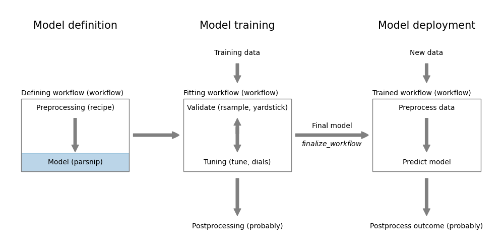
parsnip
In this section, we will learn how to train a logistic regression model using the tidymodels package. Despite its name, logistic regression is a classification model.
First, load all the packages we will need.
10.1 The UniversalBank dataset
Let’s look at the UniversalBank dataset. It is available at https://gedeck.github.io/DS-6030/datasets/UniversalBank.csv.gz. We download it using readr::read_csv.
file <-
  "https://gedeck.github.io/DS-6030/datasets/UniversalBank.csv.gz"
data <- read_csv(file)
Rows: 5000 Columns: 14
── Column specification ────────────────────────────────────────────────────────
Delimiter: ","
dbl (14): ID, Age, Experience, Income, ZIP Code, Family, CCAvg, Education, M...
ℹ Use `spec()` to retrieve the full column specification for this data.
ℹ Specify the column types or set `show_col_types = FALSE` to quiet this message.head(data)# A tibble: 6 × 14
ID Age Experience Income `ZIP Code` Family CCAvg Education Mortgage
<dbl> <dbl> <dbl> <dbl> <dbl> <dbl> <dbl> <dbl> <dbl>
1 1 25 1 49 91107 4 1.6 1 0
2 2 45 19 34 90089 3 1.5 1 0
3 3 39 15 11 94720 1 1 1 0
4 4 35 9 100 94112 1 2.7 2 0
5 5 35 8 45 91330 4 1 2 0
6 6 37 13 29 92121 4 0.4 2 155
# ℹ 5 more variables: `Personal Loan` <dbl>, `Securities Account` <dbl>,
# `CD Account` <dbl>, Online <dbl>, CreditCard <dbl>The synthetic dataset contains information about 5000 customers of a bank. The bank wants to know which customers are likely to accept a personal loan. The dataset contains 14 variables. The variable Personal Loan is the outcome variable. It is a binary variable that indicates whether the customer accepted the personal loan. The remaining variables are the predictor variables. Details can be found at https://gedeck.github.io/DS-6030/datasets/UniversalBank.html.
Next we need to preprocess the dataset:
data <- data %>%
  select(-c(ID, `ZIP Code`)) %>%
  rename(
    Personal.Loan = `Personal Loan`,
    Securities.Account = `Securities Account`,
    CD.Account = `CD Account`
  ) %>%
  mutate(
    Personal.Loan = factor(Personal.Loan, labels = c("Yes", "No"),
      levels = c(1, 0)),
    Education = factor(Education,
      labels = c("Undergrad", "Graduate", "Advanced")),
  )
str(data)  # compact representation of the data
tibble [5,000 × 12] (S3: tbl_df/tbl/data.frame)
$ Age : num [1:5000] 25 45 39 35 35 37 53 50 35 34 ...
$ Experience : num [1:5000] 1 19 15 9 8 13 27 24 10 9 ...
$ Income : num [1:5000] 49 34 11 100 45 29 72 22 81 180 ...
$ Family : num [1:5000] 4 3 1 1 4 4 2 1 3 1 ...
$ CCAvg : num [1:5000] 1.6 1.5 1 2.7 1 0.4 1.5 0.3 0.6 8.9 ...
$ Education : Factor w/ 3 levels "Undergrad","Graduate",..: 1 1 1 2 2 2 2 3 2 3 ...
$ Mortgage : num [1:5000] 0 0 0 0 0 155 0 0 104 0 ...
$ Personal.Loan : Factor w/ 2 levels "Yes","No": 2 2 2 2 2 2 2 2 2 1 ...
$ Securities.Account: num [1:5000] 1 1 0 0 0 0 0 0 0 0 ...
$ CD.Account : num [1:5000] 0 0 0 0 0 0 0 0 0 0 ...
$ Online : num [1:5000] 0 0 0 0 0 1 1 0 1 0 ...
$ CreditCard : num [1:5000] 0 0 0 0 1 0 0 1 0 0 ...The preprocessing consists of the following steps. First, we remove two columns. ID is customer specific and ZIP Code is a categorical variable with too many categories. Second, we rename the columns to remove the spaces. This makes it easier to work with the data. Third, we convert the Personal.Loan and Education variables to factors. In principle, one could convert the variables Securities.Account, CD.Account, Online, and CreditCard to factors as well. However, as they have only two levels, we will leave them as numbers.1
TipUseful to know
The outcome variable Personal.Loan is converted to a factor despite what we just said. This is important! It tells tidymodels that we want to train a classification model. If we would leave it as a number, the package would assume that we want to train a regression model. Several other packages use the same convention.
An additional advantage is that predictions will be more informative leading to easier to read predictions. In our case, the predictions will be Yes or No instead of 1 or 0.
Let’s also create a new dataset with new customers. We will use this dataset to predict whether the customer will accept a personal loan.
new_customer <- tibble(Age = 40, Experience = 10, Income = 84,
  Family = 2, CCAvg = 2, Education = 2, Mortgage = 0,
  Securities.Account = 0, CD.Account = 0, Online = 1,
  CreditCard = 1) %>%
  mutate(Education = factor(Education,
      labels = c("Undergrad", "Graduate", "Advanced"),
      levels = c(1, 2, 3)))
new_customer
# A tibble: 1 × 11
Age Experience Income Family CCAvg Education Mortgage Securities.Account
<dbl> <dbl> <dbl> <dbl> <dbl> <fct> <dbl> <dbl>
1 40 10 84 2 2 Graduate 0 0
# ℹ 3 more variables: CD.Account <dbl>, Online <dbl>, CreditCard <dbl>Note that we need to convert the Education variable to a factor. Otherwise, the prediction will fail.
10.2 Tidymodels: predicting Personal.Loan in the UniversalBank dataset
Defining and training the classification models in tidymodels is very similar to training regression models.
formula <- Personal.Loan ~ Age + Experience + Income + Family +
  CCAvg + Education + Mortgage + Securities.Account + CD.Account +
  Online + CreditCard

model <- logistic_reg() %>%
  set_engine("glm") %>%
  fit(formula, data = data)
We will use the logistic_reg() function to define a logistic regression model. The set_engine() function defines the actual model. Here it will be the glm model from base-R. We could also use set_engine("glmnet") to use the model from the glmnet package. The fit() function finally trains the model.
The result is an object of class logistic_reg. Printing the model gives details about the model.
modelparsnip model object
Call:  stats::glm(formula = Personal.Loan ~ Age + Experience + Income +
    Family + CCAvg + Education + Mortgage + Securities.Account +
    CD.Account + Online + CreditCard, family = stats::binomial,
    data = data)

Coefficients:
       (Intercept)                 Age          Experience              Income
        12.3105489           0.0359174          -0.0450379          -0.0601830
            Family               CCAvg   EducationGraduate   EducationAdvanced
        -0.6181693          -0.1633508          -3.9653781          -4.0640537
          Mortgage  Securities.Account          CD.Account              Online
        -0.0007105           0.8701362          -3.8389223           0.7605294
        CreditCard
         1.0382002

Degrees of Freedom: 4999 Total (i.e. Null);  4987 Residual
Null Deviance:      3162
Residual Deviance: 1172 AIC: 1198As we learned for the linear regression model, we can access the actual model using model$fit.
model$fit
Call: stats::glm(formula = Personal.Loan ~ Age + Experience + Income +
Family + CCAvg + Education + Mortgage + Securities.Account +
CD.Account + Online + CreditCard, family = stats::binomial,
data = data)
Coefficients:
(Intercept) Age Experience Income
12.3105489 0.0359174 -0.0450379 -0.0601830
Family CCAvg EducationGraduate EducationAdvanced
-0.6181693 -0.1633508 -3.9653781 -4.0640537
Mortgage Securities.Account CD.Account Online
-0.0007105 0.8701362 -3.8389223 0.7605294
CreditCard
1.0382002
Degrees of Freedom: 4999 Total (i.e. Null); 4987 Residual
Null Deviance: 3162
Residual Deviance: 1172 AIC: 1198Use the predict() function to predict the outcome for the new customer.
predict(model, new_data = new_customer)# A tibble: 1 × 1
.pred_class
<fct>
1 No The model predicts that the customer will not accept the loan offer. The predicted class is in the .pred_class column. Classification models can also return a probability for the prediction. Use type="prob" with the predict function.
predict(model, new_data = new_customer, type = "prob")# A tibble: 1 × 2
.pred_Yes .pred_No
<dbl> <dbl>
1 0.0109 0.989Our new customer has a very high probabily to not accept the offer; .pred_No = 0.989. The probability for the other Yes class is .pred_Yes = 0.011.
TipUseful to know
The parsnip::augment function is shortcut to predict a dataset and return a new tibble that includes the predicted values.
augment(model, new_data = new_customer)# A tibble: 1 × 14
.pred_class .pred_Yes .pred_No Age Experience Income Family CCAvg Education
<fct> <dbl> <dbl> <dbl> <dbl> <dbl> <dbl> <dbl> <fct>
1 No 0.0109 0.989 40 10 84 2 2 Graduate
# ℹ 5 more variables: Mortgage <dbl>, Securities.Account <dbl>,
# CD.Account <dbl>, Online <dbl>, CreditCard <dbl>The augment function returns a tibble that contains all the columns from the original dataset and adds the columns .pred_class and .pred_No and .pred_Yes.
10.3 Visualizing the overall model performance using a ROC curve
There are various ways of analyzing the performance of a classification model. We will discuss this in more detail in Chapter 11. Here, we will create a ROC curve to visualize the performance of our model. A ROC curve can tell you how well the model can distinguish between the two classes.
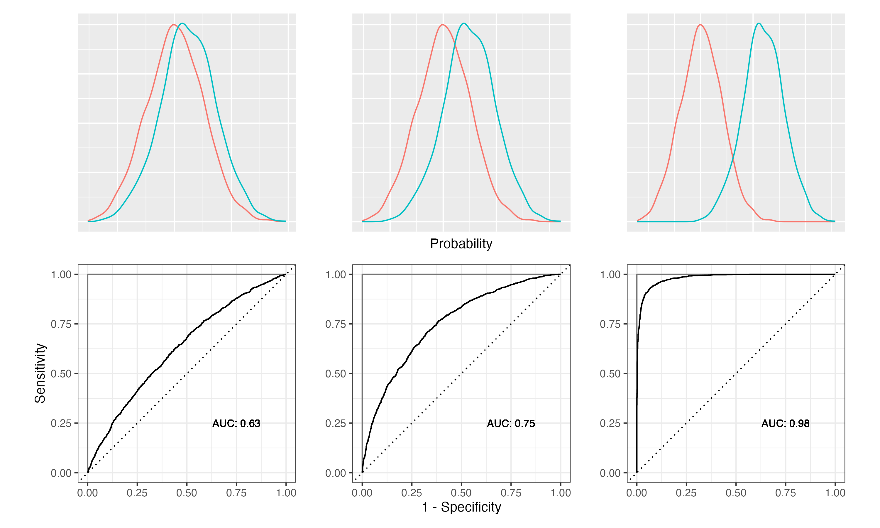
Figure 10.2 demonstrates how the class separation, the ROC curve and the AUC are related. The density plots in the top row show how the predicted probabilities are distributed for two classes. On the left, we have a model that hardly separates the two classes. On the right, the model separates the two classes very well. The corresponding ROC curves are shown in the second row. The ROC curves are the solid lines. The dashed line is the ROC curve for a random model. For the weakest model, the ROC curve is close to the random model. For the strongest model, the ROC curve gets closer and closer to the ideal model (grey lines). The AUC is the area under the ROC curve. The AUC for the weakest model is close to 0.5, which is the same as for the random model. The AUC for the strongest model is close to 1, which is the best possible value.
Let’s see how it looks like for our model. We will use yardstick::roc_curve to calculate the ROC curve.
augment(model, new_data = data) %>%
  roc_curve(Personal.Loan, .pred_Yes, event_level = "first") %>%
  autoplot()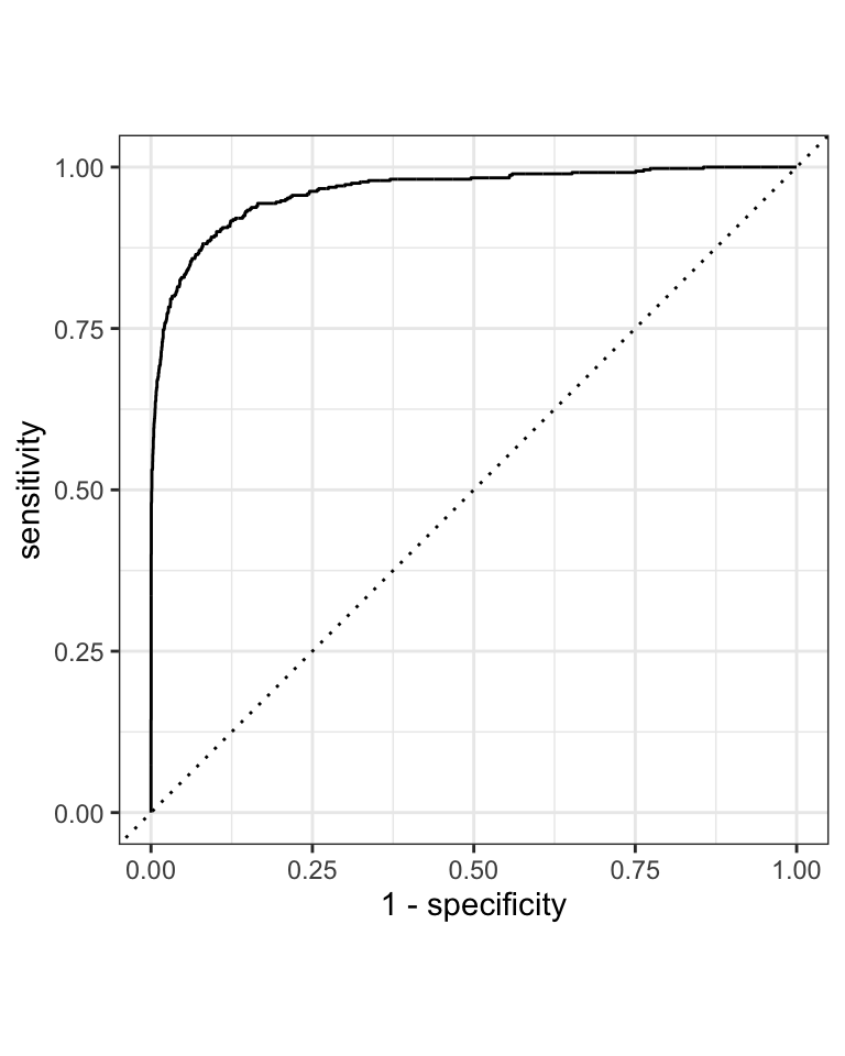
The augment() function adds the predicted class probabilities to the original dataset. This is passed into the yardstick::roc_curve function. We need to specify the actual outcome variable (Personal.Loan) and the predicted probability for the event that we are interested (.pred_Yes). The event_level argument specifies which class is the event. In our case, we are interested in the event that the customer accepts the loan. This is the first level, hence event_level="first". The roc_curve() function returns a tibble with the false positive rate (FPR) and the true positive rate (TPR). The autoplot() function creates the ROC curve as shown in Figure 10.3, but you could also use ggplot2 to create your own plot.
NoteFurther information
The tidymodels package parsnip is the package that is responsible to define and fit models. You find detailed information about each of the model types, the specific engines and their options in the documentation.
- https://parsnip.tidymodels.org/ is the documentation for the
parsnippackage. - https://parsnip.tidymodels.org/reference/ lists all the different model types that are available in
parsnip - https://parsnip.tidymodels.org/reference/logistic_reg.html is the documentation for the
logistic_reg()function. Here, you find a list of all the engines that can be used withlogistic_reg(). - https://parsnip.tidymodels.org/reference/details_logistic_reg_glm.html is the documentation for the
glmengine. These specific pages will give you more details about the different options that are available for each model.
Code
The code of this chapter is summarized here.
Show the code
knitr::opts_chunk$set(echo = TRUE, cache = TRUE, autodep = TRUE,
  fig.align = "center")
knitr::include_graphics("images/model_workflow_parsnip.png")
library(tidyverse)
library(tidymodels)
file <-
  "https://gedeck.github.io/DS-6030/datasets/UniversalBank.csv.gz"
data <- read_csv(file)
head(data)
data <- data %>%
  select(-c(ID, `ZIP Code`)) %>%
  rename(
    Personal.Loan = `Personal Loan`,
    Securities.Account = `Securities Account`,
    CD.Account = `CD Account`
  ) %>%
  mutate(
    Personal.Loan = factor(Personal.Loan, labels = c("Yes", "No"),
      levels = c(1, 0)),
    Education = factor(Education,
      labels = c("Undergrad", "Graduate", "Advanced")),
  )
str(data)  # compact representation of the data
new_customer <- tibble(Age = 40, Experience = 10, Income = 84,
  Family = 2, CCAvg = 2, Education = 2, Mortgage = 0,
  Securities.Account = 0, CD.Account = 0, Online = 1,
  CreditCard = 1) %>%
  mutate(Education = factor(Education,
      labels = c("Undergrad", "Graduate", "Advanced"),
      levels = c(1, 2, 3)))
new_customer
formula <- Personal.Loan ~ Age + Experience + Income + Family +
  CCAvg + Education + Mortgage + Securities.Account + CD.Account +
  Online + CreditCard

model <- logistic_reg() %>%
  set_engine("glm") %>%
  fit(formula, data = data)
model
model$fit
predict(model, new_data = new_customer)
predict(model, new_data = new_customer, type = "prob")
augment(model, new_data = new_customer)
knitr::include_graphics("images/roc-auc-class-separation.png")
augment(model, new_data = data) %>%
  roc_curve(Personal.Loan, .pred_Yes, event_level = "first") %>%
  autoplot()
You could convert them to make it easier to interpret the model coefficients.↩︎