library(tidymodels)
library(tidyclust)
library(kableExtra)
library(patchwork)
library(GGally)
library(DT)19 Clustering
Tidymodels provides a framework for clustering with the tidyclust package. It currently supports the following clustering algorithms:
- k-means clustering (
k_means()) - hierarchical clustering (
hier_clust())
Clustering methods are defined similarly to predictive models in tidymodels (parsnip). This means each of the methods can use different engines and we can combine we can define clustering with a preprocessing recipe in a workflow.
Load the packages we need for this chapter.
Because tuning requires training many models, we also enable parallel computing.
library(future)
plan(multisession, workers = parallel::detectCores(logical = FALSE))
19.1 k-means clustering
The k_means() function is a wrapper around four different packages. Here is an example using the default stats::kmeans engine to cluster the penguins dataset into three clusters.
# k-means clustering uses a random starting point,
# so we set a seed for reproducibility
set.seed(123)
penguins <- modeldata::penguins %>% drop_na()

formula <- ~ bill_length_mm + bill_depth_mm + flipper_length_mm +
  body_mass_g
rec_penguins <- recipe(formula, data = penguins) %>%
  step_normalize(all_predictors())
kmeans_penguins <- k_means(num_clusters = 3) %>%
  set_engine("stats") %>%
  set_mode("partition")
kmeans_wf <- workflow() %>%
  add_recipe(rec_penguins) %>%
  add_model(kmeans_penguins)
Note that the preprocessing includes a normalization step. This is recommended so that all predictors have the same scale. The kmeans_wf object can be used to fit the model.
kmeans_model <- kmeans_wf %>% fit(data = penguins)The tidy function gives us a concise overview of the results.
tidy(kmeans_model) %>% datatable(rownames = FALSE)The resulting table has a row for each cluster and contains columns for the cluster centers, the number of observations in each cluster, and the within-cluster sum of squares. The cluster center coordinates are based on normalized data and therefore not directly comparable to the original data.
TipUseful to know
It is important to set a random seed for reproducibility. The numbering of clusters as well as cluster assignments of data points in rougly equal distance to multiple cluster centers can be different each time you run the code
We can also look at the cluster center coordinates using a parallel coordinate plot (see Figure 19.1).
tidy(kmeans_model) %>%
  pivot_longer(cols = c("bill_length_mm", "bill_depth_mm",
      "flipper_length_mm", "body_mass_g")) %>%
  ggplot(aes(x = name, y = value,
      group = cluster, color = cluster, shape = cluster)) +
  geom_point(size = 3) +
  geom_line() +
  labs(x = "", y = "Value at cluster center")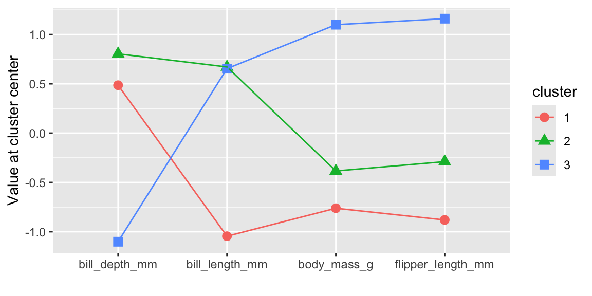
Clusters 1 and 2 have similar characteristics and differ only with respect to bill length. Cluster 1 represents penguins with smaller bill lengths compared to the penguins in clusters 2 and 3. Cluster 3 is clearly different to the other two clusters and represents penguins with a larger body mass, longer flippers, and smaller bill depth.
We can use the augment() function to add the cluster assignments to the original or new data.
cl_penguins <- augment(kmeans_model, new_data = penguins)
datatable(cl_penguins %>% head(), rownames = FALSE)
Figure 19.2 shows a scatterplot matrix (ggpairs) of the penguin data with the cluster assignments indicated by color. The clusters are clearly separated in the scatterplot matrix. The GGally package provides a ggpairs() function that can be used to create such a plot.
cl_penguins %>%
  select(-c(species, island, sex)) %>%
  ggpairs(aes(color = .pred_cluster))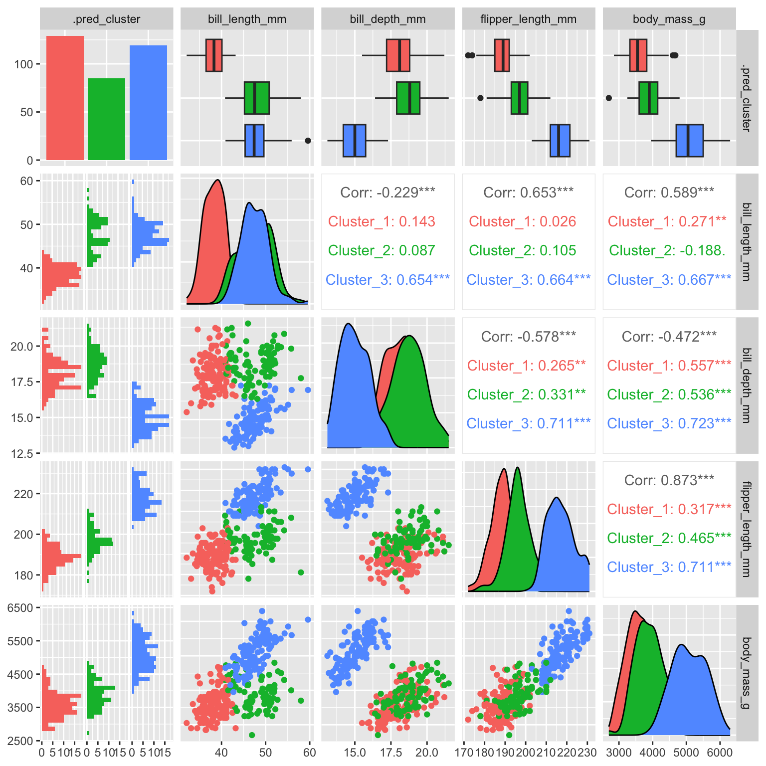
It is interesting to compare the distribution of the other variables in the clusters.
plot_distribution <- function(variable) {
  g <- ggplot(cl_penguins, aes(fill = .data[[variable]],
      x = .pred_cluster)) +
    geom_bar() +
    theme(legend.position = "inside",
      legend.position.inside = c(0.74, 0.83)) +
    scale_y_continuous(limits = c(0, 200)) +
    labs(y = "", x = "")
  return(g)
}
g1 <- plot_distribution("species")
g2 <- plot_distribution("island")
g3 <- plot_distribution("sex")

g1 + g2 + g3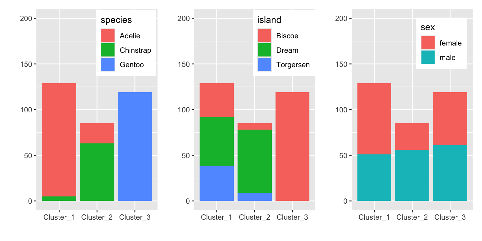
Figure 19.3 shows that the clusters separate the species well. The clusters also show some discrimination of islands. Cluster 3 contains only penguins from Biscoe and cluster 2 mostly penguins from Dream. Sex is not well separated by the clusters.
TipUseful to know
\(k\)-Means clustering requires numerical data. If your dataset contains factors, tidyclust will automatically convert these to indicator variables.1
19.2 Hierarchical clustering
The tidyclust package also provides hierarchical clustering. Using the same penguin dataset and the recipe from the previous section we can fit a hierarchical clustering as follows. In hierarchical clustering, points are combined based on distances. It is therefore recommended to normalize the data. At the time of writing, hierarchical clustering did not work as part of a workflow.2 We therefore first preprocess the data and then perform the hierarchical clustering.
formula <- ~ bill_length_mm + bill_depth_mm + flipper_length_mm +
  body_mass_g
rec_penguins <- recipe(formula, data = penguins) %>%
  step_normalize(all_predictors())

norm_penguins <- rec_penguins %>%
  prep() %>%
  bake(new_data = penguins)

hier_penguins <- hier_clust(linkage_method = "complete",
  num_clusters = 3) %>%
  set_engine("stats") %>%
  set_mode("partition")

hier_model <- hier_penguins %>% fit(formula, data = norm_penguins)
We specify the number of clusters (num_clusters) in the hier_clust function. An alternative would be to define the height at which to cut the dendrogram using cut_height.
Currently, tidyclust only provides a wrapper around the stats::hclust function. The resulting clustering can be visualized by accessing the underlying hier_model$fit object.
hier_model$fit %>% plot()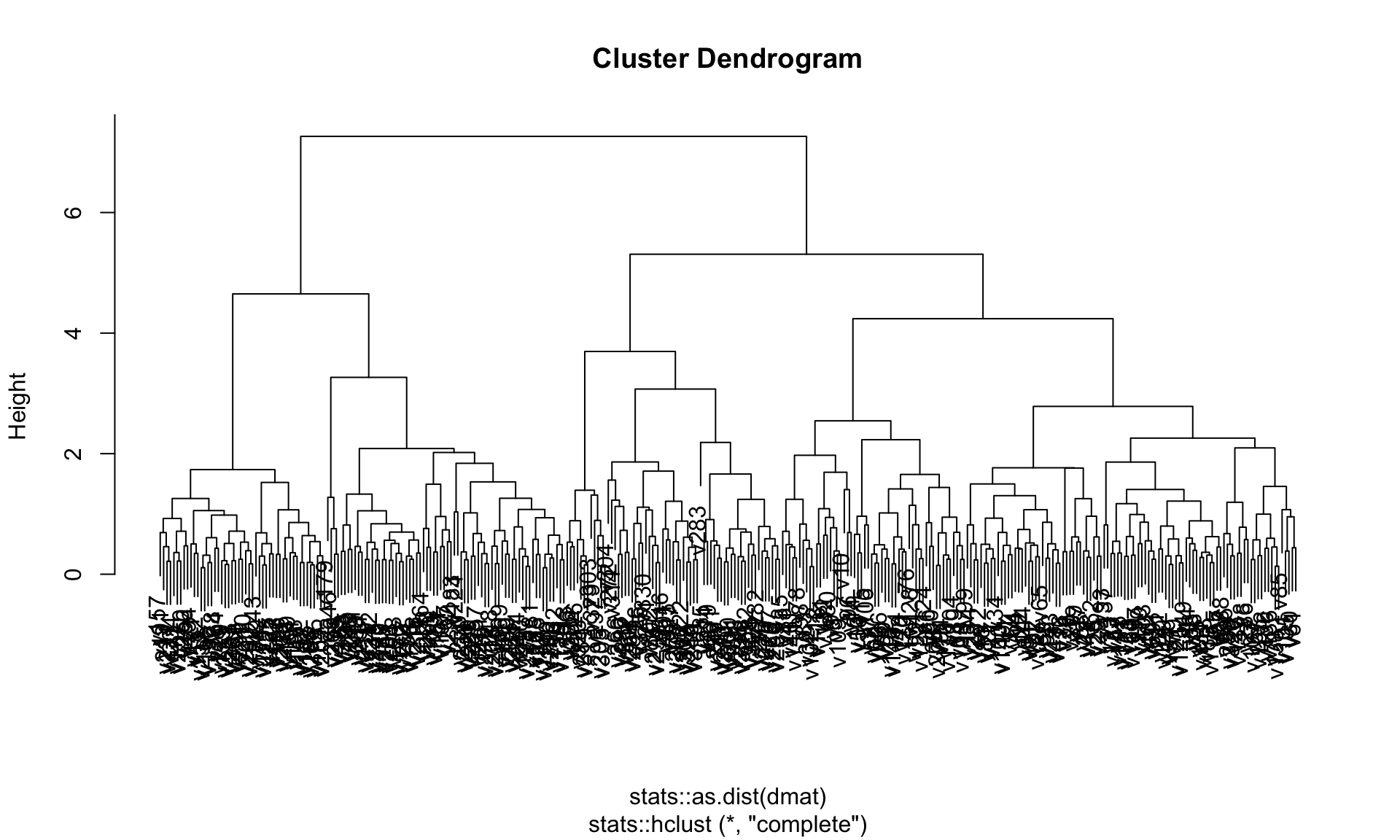
Figure 19.4 shows the dendrogram of the complete linkage clustering.
As we specified number of clusters, we can extract information about the resulting cluster.
cluster_assignment <- hier_model %>% extract_cluster_assignment()
centroids <- hier_model %>% extract_centroids()
centroids %>%
pivot_longer(cols = c("bill_length_mm", "bill_depth_mm",
"flipper_length_mm", "body_mass_g")) %>%
ggplot(aes(x = name, y = value,
group = .cluster, color = .cluster, shape = .cluster)) +
geom_point(size = 3) +
geom_line() +
labs(x = "", y = "Value at cluster center")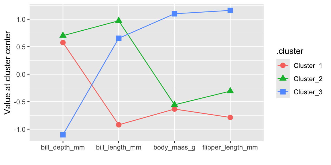
Figure 19.5 visualizes the co-ordinates of the cluster centroids. The results are comparable to the k-means clustering shown in Figure 19.1.
The resulting hiearchical clustering can also predict new data. It classifies a data point by distance to the nearest cluster centroid. In contrast to k-means clustering, you can specify the number of clusters or the cut height in the predict function.
pred_class <- hier_model %>%
predict(new_data = norm_penguins, num_clusters = 4)We can visualize the resulting cluster assignments in a pairs plot.
bind_cols(
penguins,
hier_model %>%
predict(new_data = norm_penguins, num_clusters = 4),
) %>%
select(-c(species, island, sex)) %>%
ggpairs(aes(color = .pred_cluster))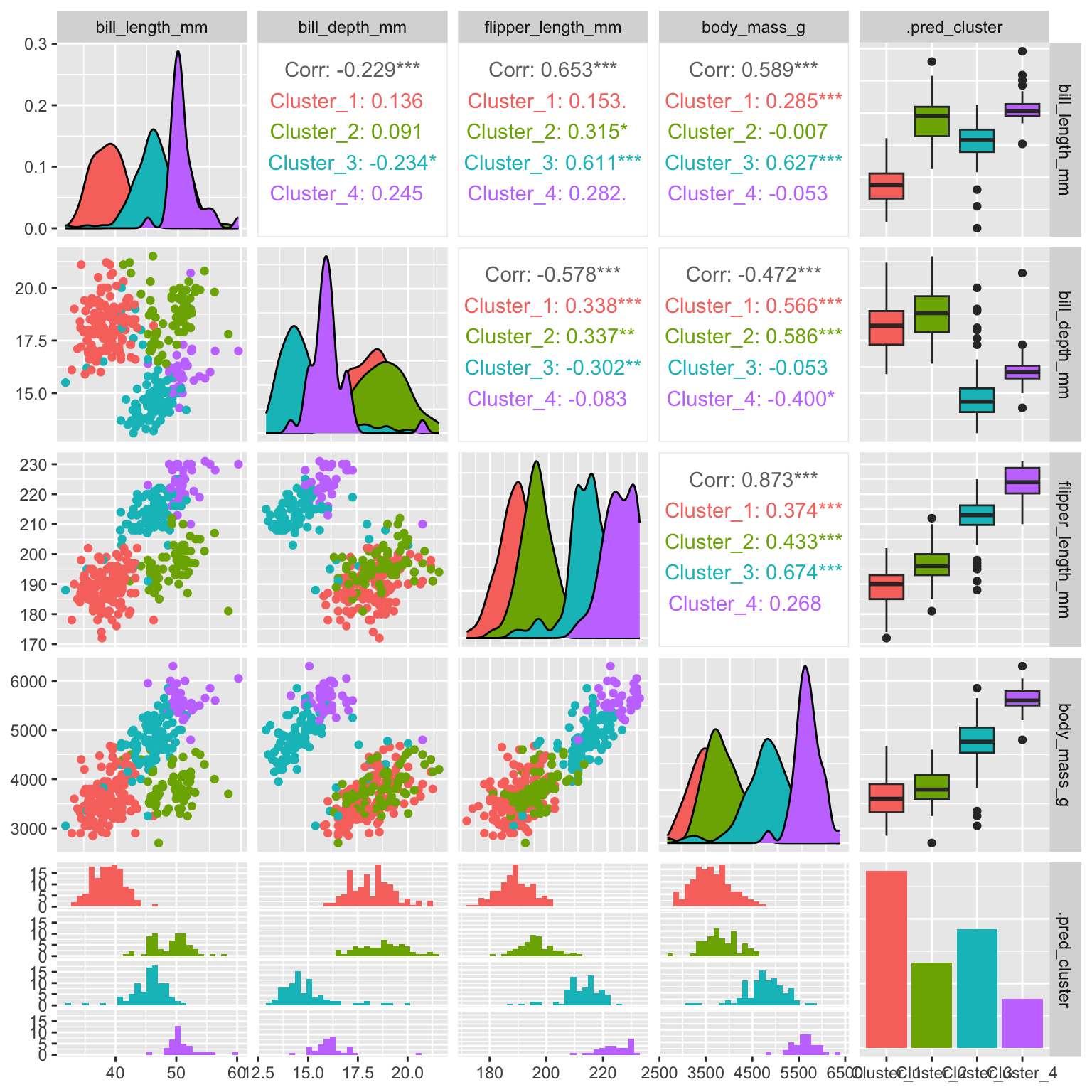
As can be seen in Figure 19.6 the additional split leads to the formation of the blue and purple clusters (compare to k-means Figure 19.2 for three clusters).
19.3 Determine the number of clusters
set.seed(123)
penguins <- modeldata::penguins %>%
drop_na()
formula <- ~ bill_length_mm + bill_depth_mm + flipper_length_mm +
body_mass_g
rec_penguins <- recipe(formula, data = penguins) %>%
step_normalize(all_predictors())
kmeans_penguins <- k_means(num_clusters = tune()) %>%
set_engine("stats") %>%
set_mode("partition")
kmeans_wf <- workflow() %>%
add_recipe(rec_penguins) %>%
add_model(kmeans_penguins)In order to tune the number of clusters, we set num_clusters=tune(). We can now run the tune_cluster function using a grid search over different values with cross-validation.
set.seed(4400)
folds <- vfold_cv(penguins, v = 2)
grid <- tibble(num_clusters = 1:10)
result <- tune_cluster(kmeans_wf, resamples = folds, grid = grid,
metrics = cluster_metric_set(sse_within_total, silhouette_avg))We can use the collect_metrics function to retrieve the cluster metrics for different cluster numbers. By default, tidyclust computes the total sum of squares (sse_total) and the within-cluster SSE (sse_within_total).
collect_metrics(result) %>% head()# A tibble: 6 × 7
num_clusters .metric .estimator mean n std_err .config
<int> <chr> <chr> <dbl> <int> <dbl> <chr>
1 1 silhouette_avg standard NaN 0 NA Preprocessor1_…
2 1 sse_within_total standard 662 2 2.00 Preprocessor1_…
3 2 silhouette_avg standard 0.529 2 0.0105 Preprocessor1_…
4 2 sse_within_total standard 278. 2 18.4 Preprocessor1_…
5 3 silhouette_avg standard 0.461 2 0.0188 Preprocessor1_…
6 3 sse_within_total standard 182. 2 1.65 Preprocessor1_…tune_cluster also supports the autoplot function to visualize the variation of cluster metrics as a function of the tuning parameter.
autoplot(result)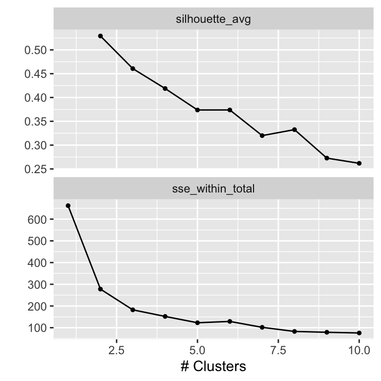
The metrics curves are interpreted as follows to determine the optimal number of clusters. For the sse_within_total curve, we look for an ellbow, a point where the slope of the curve changes visibly. In our case, the ellbow is either at 2 or at 3. In the silhouette_avg curve, the optimal cluster number corresponds to the maximum of the curve, here 2.
TipUseful to know
To identify the ellbow, sometimes also called the knee, is highly subjective. Consider the graph in Figure 19.7 again.
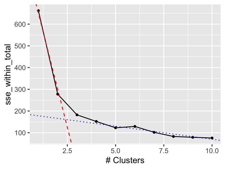
In Figure 19.8, we added two lines manually. The red, dashed line highlights the initial decline in sse_within_total and the blue, dotted line the later, less rapid change. The two lines cross around 2.5 (the ellbow) which tells us that we should use 2 or 3 clusters.
While approaches like the ellbow method or metrics like the silhouette_avg can act as a guideline, the decision of how many clusters to keep is somewhat subjective and often depends more on the use case.
Once we have made a decision on the number of clusters, we can train a finalized model using the finalize_model_tidyclust or finalize_workflow_tidyclust methods.
best_params <- data.frame(num_clusters = 3)
model <- finalize_workflow_tidyclust(kmeans_wf, best_params)
model══ Workflow ════════════════════════════════════════════════════════════════════
Preprocessor: Recipe
Model: k_means()
── Preprocessor ────────────────────────────────────────────────────────────────
1 Recipe Step
• step_normalize()
── Model ───────────────────────────────────────────────────────────────────────
K Means Cluster Specification (partition)
Main Arguments:
num_clusters = 3
Computational engine: stats
NoteFurther information
- https://tidyclust.tidymodels.org/
tidyclustpackage
Code
The code of this chapter is summarized here.
Show the code
knitr::opts_chunk$set(echo = TRUE, cache = TRUE, autodep = TRUE,
fig.align = "center")
library(tidymodels)
library(tidyclust)
library(kableExtra)
library(patchwork)
library(GGally)
library(DT)
library(future)
plan(multisession, workers = parallel::detectCores(logical = FALSE))
# k-means clustering uses a random starting point,
# so we set a seed for reproducibility
set.seed(123)
penguins <- modeldata::penguins %>% drop_na()
formula <- ~ bill_length_mm + bill_depth_mm + flipper_length_mm +
body_mass_g
rec_penguins <- recipe(formula, data = penguins) %>%
step_normalize(all_predictors())
kmeans_penguins <- k_means(num_clusters = 3) %>%
set_engine("stats") %>%
set_mode("partition")
kmeans_wf <- workflow() %>%
add_recipe(rec_penguins) %>%
add_model(kmeans_penguins)
kmeans_model <- kmeans_wf %>% fit(data = penguins)
tidy(kmeans_model) %>% datatable(rownames = FALSE)
tidy(kmeans_model) %>%
pivot_longer(cols = c("bill_length_mm", "bill_depth_mm",
"flipper_length_mm", "body_mass_g")) %>%
ggplot(aes(x = name, y = value,
group = cluster, color = cluster, shape = cluster)) +
geom_point(size = 3) +
geom_line() +
labs(x = "", y = "Value at cluster center")
cl_penguins <- augment(kmeans_model, new_data = penguins)
datatable(cl_penguins %>% head(), rownames = FALSE)
cl_penguins %>%
select(-c(species, island, sex)) %>%
ggpairs(aes(color = .pred_cluster))
plot_distribution <- function(variable) {
g <- ggplot(cl_penguins, aes(fill = .data[[variable]],
x = .pred_cluster)) +
geom_bar() +
theme(legend.position = "inside",
legend.position.inside = c(0.74, 0.83)) +
scale_y_continuous(limits = c(0, 200)) +
labs(y = "", x = "")
return(g)
}
g1 <- plot_distribution("species")
g2 <- plot_distribution("island")
g3 <- plot_distribution("sex")
g1 + g2 + g3
formula <- ~ bill_length_mm + bill_depth_mm + flipper_length_mm +
body_mass_g
rec_penguins <- recipe(formula, data = penguins) %>%
step_normalize(all_predictors())
norm_penguins <- rec_penguins %>%
prep() %>%
bake(new_data = penguins)
hier_penguins <- hier_clust(linkage_method = "complete",
num_clusters = 3) %>%
set_engine("stats") %>%
set_mode("partition")
hier_model <- hier_penguins %>% fit(formula, data = norm_penguins)
hier_model$fit %>% plot()
cluster_assignment <- hier_model %>% extract_cluster_assignment()
centroids <- hier_model %>% extract_centroids()
centroids %>%
  pivot_longer(cols = c("bill_length_mm", "bill_depth_mm",
      "flipper_length_mm", "body_mass_g")) %>%
  ggplot(aes(x = name, y = value,
      group = .cluster, color = .cluster, shape = .cluster)) +
  geom_point(size = 3) +
  geom_line() +
  labs(x = "", y = "Value at cluster center")
pred_class <- hier_model %>%
  predict(new_data = norm_penguins, num_clusters = 4)
bind_cols(
  penguins,
  hier_model %>%
    predict(new_data = norm_penguins, num_clusters = 4),
) %>%
  select(-c(species, island,  sex)) %>%
  ggpairs(aes(color = .pred_cluster))
set.seed(123)
penguins <- modeldata::penguins %>%
  drop_na()

formula <- ~ bill_length_mm + bill_depth_mm + flipper_length_mm +
  body_mass_g
rec_penguins <- recipe(formula, data = penguins) %>%
  step_normalize(all_predictors())
kmeans_penguins <- k_means(num_clusters = tune()) %>%
  set_engine("stats") %>%
  set_mode("partition")
kmeans_wf <- workflow() %>%
  add_recipe(rec_penguins) %>%
  add_model(kmeans_penguins)
set.seed(4400)
folds <- vfold_cv(penguins, v = 2)
grid <- tibble(num_clusters = 1:10)
result <- tune_cluster(kmeans_wf, resamples = folds, grid = grid,
  metrics = cluster_metric_set(sse_within_total, silhouette_avg))
collect_metrics(result) %>% head()
autoplot(result)
autoplot(result, metric = "sse_within_total") +
geom_abline(intercept = 1000, slope = -350, linetype = "dashed",
color = "red") +
geom_abline(intercept = 190, slope = -12, linetype = "dotted",
color = "blue")
best_params <- data.frame(num_clusters = 3)
model <- finalize_workflow_tidyclust(kmeans_wf, best_params)
model