library(tidyverse)
library(tidymodels)
library(kableExtra)
library(ggfortify)  # required for diagnostics plots
library(DT)20 Linear regression models
The DS-6030 course primarily focuses on predictive modeling. However, it is useful to know how to access the model parameters and interpret them for linear regression models. In this section, we will use the tidymodels framework to build a linear regression model and then look at the model parameters and diagnostics.
Load required libraries
20.1 Build a linear regression model
We will use the example from Chapter 8 here.
data <- datasets::mtcars %>%
  as_tibble(rownames = "car") %>%
  mutate(
    vs = factor(vs, labels = c("V-shaped", "straight")),
    am = factor(am, labels = c("automatic", "manual")),
  )
formula <- mpg ~ cyl + disp + hp + drat + wt + qsec + vs + am +
  gear + carb
model <- linear_reg(engine = "lm", mode = "regression") %>%
  fit(formula, data = data)
20.2 Analyze model parameters
The tidyverse framework introduced the function tidy which is a generic function similar to plot or predict. This means, there are implementations for objects of different types. The parsnip package also provides an implementations of the tidy function that, works for fitted models. Using it with our linear regression model, extracts the model parameters. Table 20.1 shows the model parameters extracted with the tidy function.
model %>%
  tidy() %>%
  datatable(rownames = FALSE) %>%
  formatRound(
    columns = c("estimate", "std.error", "statistic", "p.value"),
    digits = 3
)20.3 Extract model statistics
The broom package provides the function glance to extract model statistics from a fitted linear regression model. Table 20.2 shows the model statistics for our case.
model %>%
  glance() %>%
  datatable(rownames = FALSE) %>%
formatRound(columns = names(model %>% glance()), digits = 3)20.4 Diagnostics plots
The ggfortify package provides implementations of the generic autoplot function that creates up to six diagnostics plots using ggplot. The plots are selected using the which argument. The default creates four plots (1, 2, 3, and 5).
| which | Plot |
|---|---|
| 1 | Residuals vs Fitted |
| 2 | Normal Q-Q |
| 3 | Scale-Location |
| 4 | Cook's distance |
| 5 | Residuals vs Leverage |
| 6 | Cooks's distance vs Leverage |
Plots created by `which` argument
20.4.1 Residuals vs Fitted
The argument which=1 creates a graph of residuals vs fitted (see Figure 20.1). This type of plot is useful for all types of regression, not only linear regressions models.
autoplot(model, which = c(1, 2))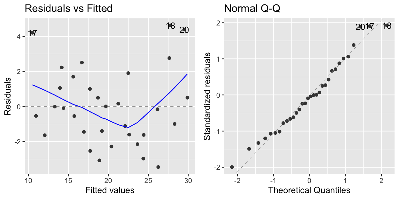
which=1) and Normal Q-Q plot (which=2)
The blue line is a smoother of the residuals. The line should be a flat line and show no trend in the data. Looking at the plot, we can see that there is some non-linearity in the residuals. This could be an indication to explore variable transformations or polynomial terms.
The plot can also reveal heteroscedasticity of the residuals. It is however more qualitative; the scale-location plot can show this better.
20.4.2 Normal Q-Q plot
The normal Q-Q plot looks at the distribution of the residuals. The normal Q-Q plot in Figure 20.1 shows that in our case, residuals are normally distributed.
20.4.3 Scale-location plot
autoplot(model, which = c(3, 4))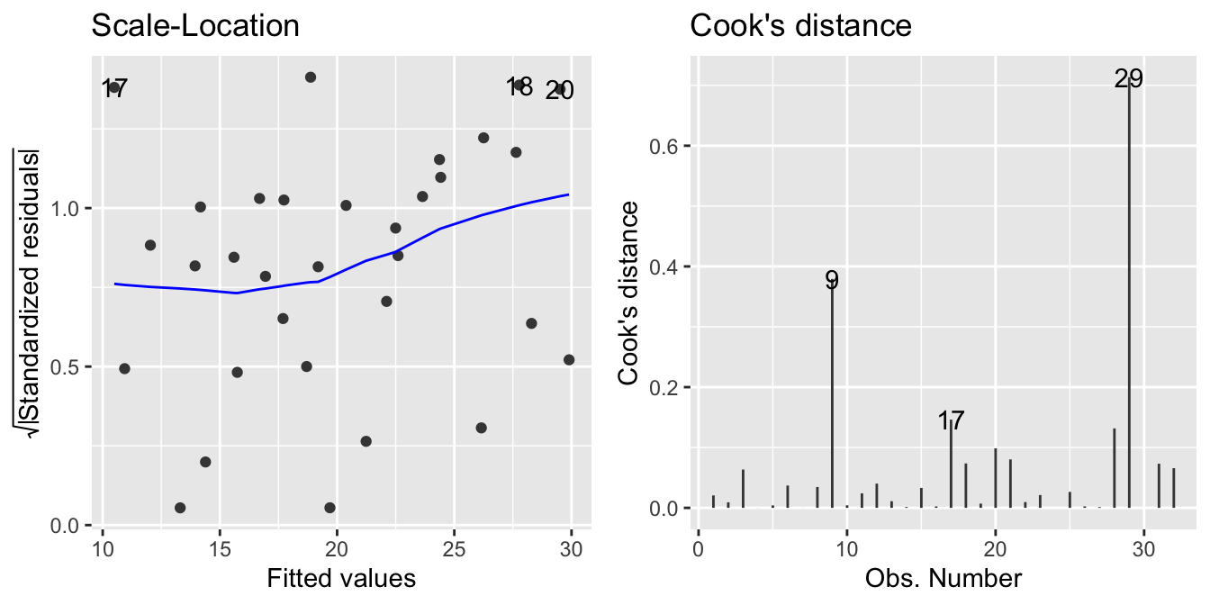
which=3) and Cook’s distance plot (which=4)
The scale location plot can reveal changes in variance of the residuals easier. Figure 20.2, shows that in our case, the variation doesn’t change much.
20.4.4 Cook’s distance plot
The Cook’s distance measures the influence of a data point on the regression. Figure 20.2, shows that two data points stand out (9 and 29).
Some suggest that points with a Cook’s distance greater than 1 should be looked at. None of our data points are flagged in this case. Others suggest \(4/(n-p-1)\) as a threshold. For our model, \(n=32\) and \(p=10\), so \(4/(n-p-1) = 4/(32-10-1) = 0.19\). This will flag 9 and 29 as points of interest.
20.4.5 Residuals vs Leverage
autoplot(model, which = c(5, 6))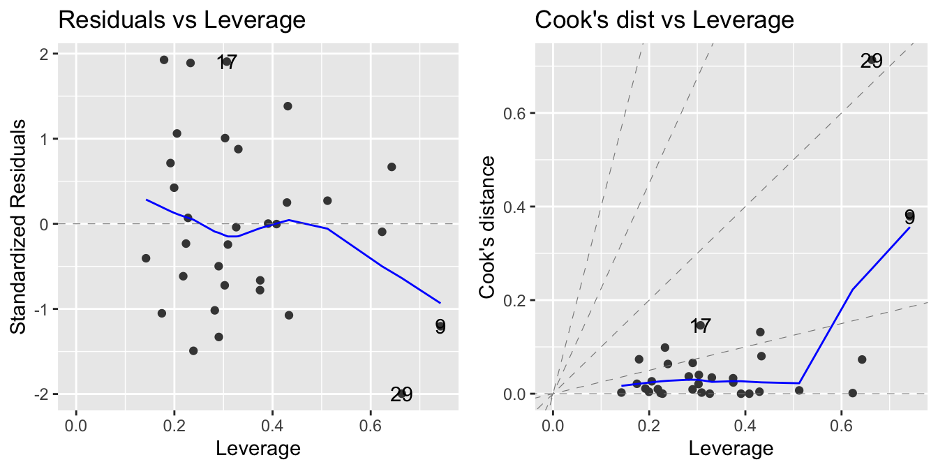
which=5) and Cook’s distance vs leverage (which=6)
Leverage is another measure of how influential a data point is. The larger the leverage, the more the data point affects the regression. In our case (see Figure 20.3), no point stands out.
20.4.6 Cooks’s distance vs Leverage
The final plot shows Cook’s distance vs leverage (see Figure 20.3). Again, look for points with large Cook’s distance or large leverage.
NoteFurther information
Additional information can be found in the following resources:
- https://bookdown.org/dereksonderegger/571/7-Diagnostics-Chapter.html
- Comprehensive slide deck by John Fox, the author of the book “Regression Diagnostics” https://socialsciences.mcmaster.ca/jfox/Courses/Brazil-2009/slides-handout.pdf
Code
The code of this chapter is summarized here.
Show the code
knitr::opts_chunk$set(echo = TRUE, cache = TRUE, autodep = TRUE,
  fig.align = "center")
library(tidyverse)
library(tidymodels)
library(kableExtra)
library(ggfortify)  # required for diagnostics plots
library(DT)
data <- datasets::mtcars %>%
  as_tibble(rownames = "car") %>%
  mutate(
    vs = factor(vs, labels = c("V-shaped", "straight")),
    am = factor(am, labels = c("automatic", "manual")),
  )
formula <- mpg ~ cyl + disp + hp + drat + wt + qsec + vs + am +
  gear + carb
model <- linear_reg(engine = "lm", mode = "regression") %>%
  fit(formula, data = data)
model %>%
  tidy() %>%
  datatable(rownames = FALSE) %>%
  formatRound(
    columns = c("estimate", "std.error", "statistic", "p.value"),
    digits = 3
  )
model %>%
  glance() %>%
  datatable(rownames = FALSE) %>%
  formatRound(columns = names(model %>% glance()), digits = 3)
tibble(
  which = c(1, 2, 3, 4, 5, 6),
  Plot = c("Residuals vs Fitted", "Normal Q-Q",
    "Scale-Location", "Cook's distance",
    "Residuals vs Leverage", "Cooks's distance vs Leverage")
) %>%
  kableExtra::kbl(caption = "Plots created by `which` argument") %>%
  kableExtra::kable_styling(full_width = FALSE)
autoplot(model, which = c(1, 2))
autoplot(model, which = c(3, 4))
autoplot(model, which = c(5, 6))