25 Model tuning

In this example, we will

load and preprocess data
define a workflow with tunable parameters
tune the hyperparameters using Bayesian optimization
train the final model
evaluate the model using cross-validation and holdout data

using the Loan prediction dataset to illustrate the whole process.

Load the required packages:

library(tidyverse)
library(tidymodels)

Load and preprocess the data:

file <- "https://gedeck.github.io/DS-6030/datasets/loan_prediction.csv"
data <- read_csv(file, show_col_types = FALSE) %>%
  drop_na() %>%
  mutate(
    Gender = as.factor(Gender),
    Married = as.factor(Married),
    Dependents = gsub("\\+", "", Dependents) %>% as.numeric(),
    Education = as.factor(Education),
    Self_Employed = as.factor(Self_Employed),
    Credit_History = as.factor(Credit_History),
    Property_Area = as.factor(Property_Area),
    Loan_Status = factor(Loan_Status, levels = c("N", "Y"),
      labels = c("No", "Yes"))
  ) %>%
  select(-Loan_ID)

Split dataset into training and holdout data, prepare for cross-validation:

set.seed(123)
data_split <- initial_split(data, prop = 0.8, strata = Loan_Status)
train_data <- training(data_split)
holdout_data <- testing(data_split)

resamples <- vfold_cv(train_data, v = 10, strata = Loan_Status)
cv_metrics <- metric_set(roc_auc, accuracy)
cv_control <- control_resamples(save_pred = TRUE)

Define the recipe, the model specification (elasticnet logistic regression), and combine them into a workflow:

formula <- Loan_Status ~ Gender + Married + Dependents + Education +
  Self_Employed + ApplicantIncome + CoapplicantIncome + LoanAmount +
  Loan_Amount_Term + Credit_History + Property_Area
recipe_spec <- recipe(formula, data = train_data) %>%
  step_dummy(all_nominal(), -all_outcomes())

model_spec <- logistic_reg(engine = "glmnet", mode = "classification",
  penalty = tune(), mixture = tune())

wf <- workflow() %>%
  add_model(model_spec) %>%
  add_recipe(recipe_spec)

Tune the penalty and mixture hyperparameters using Bayesian hyperparameter optimization:

parameters <- extract_parameter_set_dials(wf) %>%
  update(penalty = penalty(c(-4, -1)))
tune_wf <- tune_bayes(wf, resamples = resamples, metrics = cv_metrics,
  param_info = parameters, iter = 25)

! No improvement for 10 iterations; returning current results.

The autoplot of the tune_bayes object (Figure 25.1) shows the ROC-AUC for different values of the penalty and mixture hyperparameters. We can see that the best roc_auc is obtained with penalty and mixture values inside the tuning range. We don’t need to adjust the sampling ranges for the hyperparameters.

autoplot(tune_wf)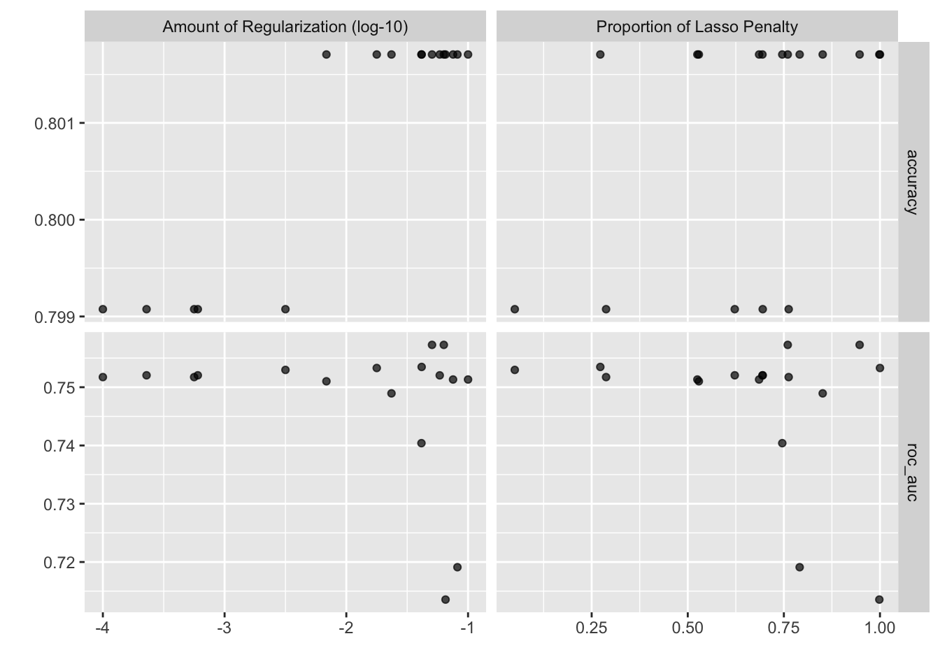

Figure 25.1: Autoplot shows the ROC-AUC for different values of the penalty and mixture hyperparameters.

Finalize the workflow:

best_parameter <- select_best(tune_wf, metric = "roc_auc")
best_wf <- finalize_workflow(wf, best_parameter)

The best roc_auc is obtained with a penalty of best_parameter['penalty'] = 0.0632251 and a mixture of best_parameter['mixture'] = 0.7600721.

Use the tuned workflow for cross-validation and training the final model using the full dataset:

result_cv <-  fit_resamples(best_wf, resamples,
  metrics = cv_metrics, control = cv_control)
fitted_model <- best_wf %>% fit(train_data)

Estimate model performance using the cross-validation results and the holdout data:

cv_results <- collect_metrics(result_cv) %>%
  select(.metric, mean) %>%
  rename(.estimate = mean) %>%
  mutate(result = "Cross-validation")
holdout_predictions <- augment(fitted_model, new_data = holdout_data)
holdout_results <-  bind_rows(
  c(roc_auc(holdout_predictions, Loan_Status, .pred_Yes,
      event_level = "second")),
  c(accuracy(holdout_predictions, Loan_Status, .pred_class))
) %>%
  select(-.estimator) %>%
  mutate(result = "Holdout")

The performance metrics are summarized in the following table.

bind_rows(
  cv_results,
  holdout_results
) %>%
  pivot_wider(names_from = .metric, values_from = .estimate) %>%
  kableExtra::kbl(caption = "Model performance metrics", digits = 3) %>%
  kableExtra::kable_styling(full_width = FALSE)

result	accuracy	roc_auc
Cross-validation	0.802	0.757
Holdout	0.835	0.741

Model performance metrics

Code

The code of this chapter is summarized here.

Show the code

knitr::opts_chunk$set(echo = TRUE, cache = TRUE, autodep = TRUE,
  fig.align = "center")
library(tidyverse)
library(tidymodels)
file <- "https://gedeck.github.io/DS-6030/datasets/loan_prediction.csv"
data <- read_csv(file, show_col_types = FALSE) %>%
  drop_na() %>%
  mutate(
    Gender = as.factor(Gender),
    Married = as.factor(Married),
    Dependents = gsub("\\+", "", Dependents) %>% as.numeric(),
    Education = as.factor(Education),
    Self_Employed = as.factor(Self_Employed),
    Credit_History = as.factor(Credit_History),
    Property_Area = as.factor(Property_Area),
    Loan_Status = factor(Loan_Status, levels = c("N", "Y"),
      labels = c("No", "Yes"))
  ) %>%
  select(-Loan_ID)
set.seed(123)
data_split <- initial_split(data, prop = 0.8, strata = Loan_Status)
train_data <- training(data_split)
holdout_data <- testing(data_split)

resamples <- vfold_cv(train_data, v = 10, strata = Loan_Status)
cv_metrics <- metric_set(roc_auc, accuracy)
cv_control <- control_resamples(save_pred = TRUE)
formula <- Loan_Status ~ Gender + Married + Dependents + Education +
  Self_Employed + ApplicantIncome + CoapplicantIncome + LoanAmount +
  Loan_Amount_Term + Credit_History + Property_Area
recipe_spec <- recipe(formula, data = train_data) %>%
  step_dummy(all_nominal(), -all_outcomes())

model_spec <- logistic_reg(engine = "glmnet", mode = "classification",
  penalty = tune(), mixture = tune())

wf <- workflow() %>%
  add_model(model_spec) %>%
  add_recipe(recipe_spec)
parameters <- extract_parameter_set_dials(wf) %>%
  update(penalty = penalty(c(-4, -1)))
tune_wf <- tune_bayes(wf, resamples = resamples, metrics = cv_metrics,
  param_info = parameters, iter = 25)
autoplot(tune_wf)
best_parameter <- select_best(tune_wf, metric = "roc_auc")
best_wf <- finalize_workflow(wf, best_parameter)
result_cv <-  fit_resamples(best_wf, resamples,
  metrics = cv_metrics, control = cv_control)
fitted_model <- best_wf %>% fit(train_data)
cv_results <- collect_metrics(result_cv) %>%
  select(.metric, mean) %>%
  rename(.estimate = mean) %>%
  mutate(result = "Cross-validation")
holdout_predictions <- augment(fitted_model, new_data = holdout_data)
holdout_results <-  bind_rows(
  c(roc_auc(holdout_predictions, Loan_Status, .pred_Yes,
      event_level = "second")),
  c(accuracy(holdout_predictions, Loan_Status, .pred_class))
) %>%
  select(-.estimator) %>%
  mutate(result = "Holdout")
bind_rows(
  cv_results,
  holdout_results
) %>%
  pivot_wider(names_from = .metric, values_from = .estimate) %>%
  kableExtra::kbl(caption = "Model performance metrics", digits = 3) %>%
  kableExtra::kable_styling(full_width = FALSE)