14 Model tuning - the basics

In the previous chapters, we learned how to define data preprocessing steps, select a specific model type, train the model and validate its performance. In this chapter, we will learn how to tune our models to get the best performance out of them.

There are many ways a model can be tuned.

Feature engineering: Feature engineering is the process of creating new features from existing features. This can be as simple as replacing a feature with its square root value, or can involve combining several features. We will learn more about feature engineering in Section 15.1.
Regularization: Regularization is a technique used to prevent overfitting in models. It involves adding a penalty term to the loss function used to train the model. We will learn more about regularization in Section 15.2.
Feature selection: Feature selection is the process of selecting the most important features for a given model. We will learn more about feature selection in Section 15.3.
Hyperparameter tuning: Hyperparameters are parameters that are not learned during the training process. Instead, they are set before the training process starts. For example, the number of neighbors in a k-nearest neighbor model is a hyperparameter. Hyperparameter tuning is the process of finding the best hyperparameter values for a given model type. We will learn more about hyperparameter tuning in this Chapter and in Section 15.4.
Threshold selection: Threshold selection is the process of finding the best threshold for a given classification model. This is currently not included in the workflow package, but can be done post-training using the probably package (see Section 11.1.2).

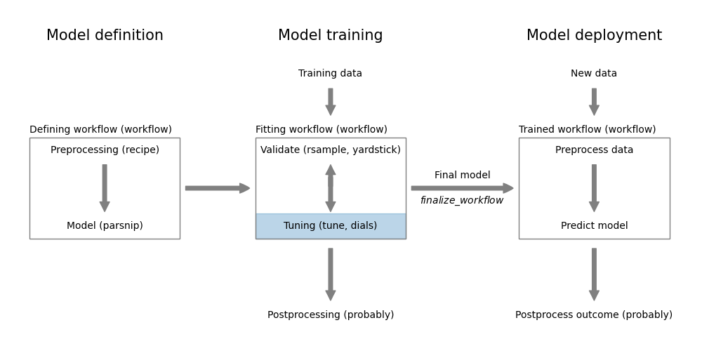
Figure 14.1 shows how this step fits into the overall model workflow.

Load the packages we need for this chapter.

library(tidymodels)

14.1 Specifying tunable parameters

In the tidymodels framework, the tune package has the task of optimizing models using tuning. To do this, it needs to know what should be tuned. We can specify tunable parameters in the preprocessing steps defined using recipe objects and in the model definition step using parsnip objects.

For example, for principal component regression, we want to select the number of principal components to use in the regression model. The step_pca function has the num_comp argument that specifies the number of principal components to use. If we want to find the optimal value of num_comp, we specify this as a tuning parameter using the tune() function in the recipe.

mtcars_rec <- recipe(mpg ~ ., data = mtcars) %>%
  step_normalize(all_numeric_predictors()) %>%
  step_pca(all_numeric_predictors(), num_comp = tune())

Another example, is the number of neighbors in a $k$-nearest neighbor model. We can specify this number in the nearest_neighbor() function using the neighbors argument.

model <- nearest_neighbor(mode = "regression", neighbors = tune())

By combining the recipe and model into a workflow, we define a k-nearest neighbor model using principal components where we optimize both the number of components and the number of neighbors.

mtcars_workflow <- workflow() %>%
  add_recipe(mtcars_rec) %>%
  add_model(model)
parameters <- extract_parameter_set_dials(mtcars_workflow)
parameters %>% knitr::kable()

name	id	source	component	component_id	object
neighbors	neighbors	model_spec	nearest_neighbor	main	integer , 1 , 15 , TRUE , TRUE , # Nearest Neighbors
num_comp	num_comp	recipe	step_pca	pca_AHvGb	integer, 1, 4, TRUE, TRUE, # Components, function (object, x, log_vals = FALSE, …) , {, check_param(object), rngs <- range_get(object, original = FALSE), if (!is_unknown(rngs$upper)) {, return(object), }, x_dims <- dim(x), if (is.null(x_dims)) {, cli::cli_abort("Cannot determine number of columns. Is {.arg x} a 2D data object?"), }, if (log_vals) {, rngs[2] <- log10(x_dims[2]), }, else {, rngs[2] <- x_dims[2], }, if (object$type == “integer” & is.null(object$trans)) {, rngs <- as.integer(rngs), }, range_set(object, rngs), }

The extract_parameter_set_dials function tells us that the workflow has two tunable parameters: num_comp and neighbors. The table also informs us where the parameters are used: neighbors is used in the nearest_neighbor function and num_comp is used in the step_pca function. Most importantly, it identifies the type of tuning that is used for each parameter. The name column tells us the function from the dials package that is used to optimize the parameter; see the dials documentation for more information.

The object column contains the actual definition of the search space of the parameter. Let’s have a look at the default settings.

parameters$object[1]

[[1]]

# Nearest Neighbors (quantitative)

Range: [1, 15]

parameters$object[2]

[[1]]

# Components (quantitative)

Range: [1, 4]

The number of components in the PCA can range between 1 and 4, the number of neighbors between 1 and 15. This may not be suitable for our problem and it often isn’t. We can change the settings for one or more of the tunable parameters using the update function.

parameters <- parameters %>%
  update(
    num_comp = num_comp(c(1, 10)),
    neighbors = neighbors(c(1, 5)),
  )

This increases the search range for number of components from 1 to 10 and reduces the search space for neighbors from 1 to 5.

Useful to know

If you have multiple tuning parameters in your workflow of the same type, you identify them using an identifier in the tune function, e.g. tune("pca1") and tune("pca2"). You can then modify the default settings for each of them separately, e.g.

parameter_set <- parameter_set %>%
  update(
    pca1 = num_comp(10, 30),
    pca2 = num_comp(1, 5),
  )

14.2 Data-specific tuning parameters

The previous section we used the number of neighbors as an example. While in principle it could be set to a value larger than the number of data points in the training set, realistically the value of the tuning parameter will always be in a range that is independent of the data set. ¹

However, there are tuning parameters, where the range can be dependent on the number of features. Some tuning parameters have a data-specific component. For example, in random forests (see Section A.12), we can control the number of features that are evaluated at each split of the decision trees with the mtry parameter. This value can range between 1 and the number of features in the dataset after preprocessing. The upper bound of this value is therefore unknown and needs to be explicitly set. Tidymodel will let you know when this is the case. Let’s look at the random forest case:

wf <- workflow() %>%
  add_recipe(mtcars_rec) %>%
  add_model(rand_forest(mtry = tune(), mode = "regression"))
p <- extract_parameter_set_dials(wf)
p

Collection of 2 parameters for tuning

 identifier     type    object
       mtry     mtry nparam[?]
   num_comp num_comp nparam[+]

Model parameters needing finalization:

# Randomly Selected Predictors ('mtry')

See `?dials::finalize()` or `?dials::update.parameters()` for more information.

The output tells us that some

Model parameters needing finalization:
# Randomly Selected Predictors ('mtry')

We can find out more about this by inspecting p$object[[1]].

p$object[[1]]

# Randomly Selected Predictors (quantitative)

Range: [1, ?]

The range for the mtry parameter is defined as [1, ?] where ? indicates that the upper bound is unspecified. If we use the parameters as they are, tuning will throw an error.

grid_regular(p)

Error in `grid_regular()`:
! These arguments contain unknowns: `mtry`.
ℹ See the `finalize()` function.

We need to specify the upper bound for the mtry parameter. This can be done by setting a range using dials::update_parameters in the same way as we did for other parameters in Section 14.1. Alternatively, we can use the dials::finalize function as follows:

p <- extract_parameter_set_dials(wf) %>%
  finalize(mtcars %>% select(-mpg))
p$object[[1]]

# Randomly Selected Predictors (quantitative)

Range: [1, 10]

The range for the mtry parameter is now defined as [1, 10].

14.3 Tuning a workflow

Now that we have specified the tuning parameters, we can use them to search our parameter space to identify the best model.

set.seed(123)
tune_results <- tune_grid(mtcars_workflow,
  resamples = vfold_cv(mtcars), grid = grid_regular(parameters))

The tune_grid function requires the workflow, information about the validation strategy (resamples) and the search space (grid). With the exception of the grid argument, this is very similar to the fit_resamples function that we encountered in Chapter 13. For each combination of tuning parameters defined in the grid argument, the tune_grid function trains a model and evaluates its performance.

The grid argument specifies the search space for the tuning parameters. In this case, we use a regular grid search. We will learn more about grid search strategies in Section 14.4.

Printing the tune_results object is not very informative. The output will only tell us that it’s a tibble with tuning results for a 10-fold cross valiation. The tibble contains the tuning parameters and the performance metrics for each model and cross-validation fold.

You can visualize the results using the autoplot function:

autoplot(tune_results)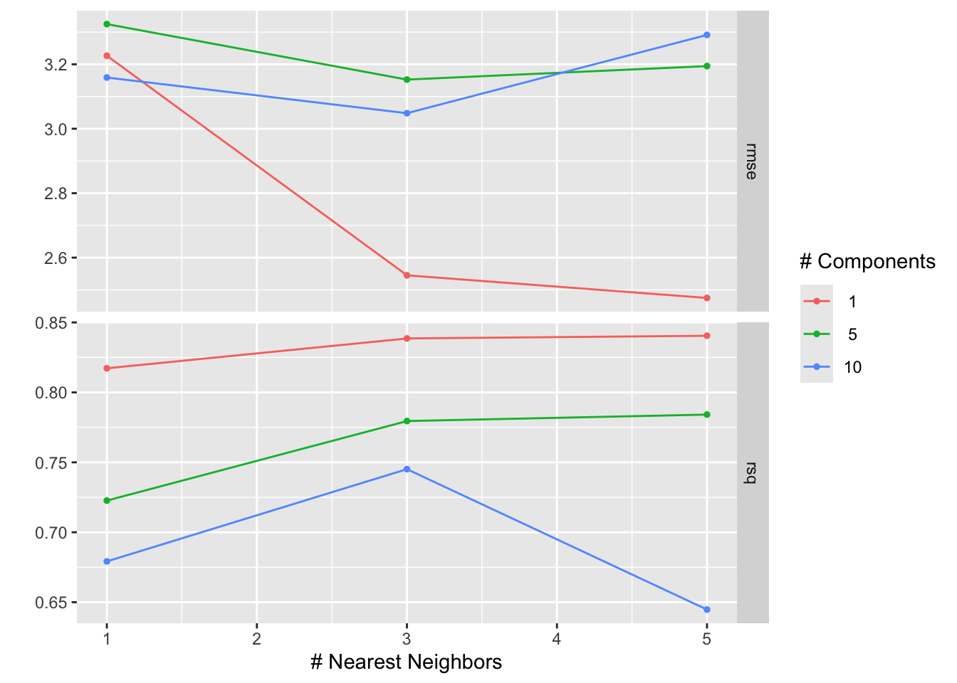

Figure 14.2: Visualization of tuning results for workflow tuning

Figure 14.2 shows the results of the tuning process. The $x$-axis shows the number of neighbors in the $k$-nearest neighbor model and the $y$-axis the values of the two calculated metrics, rmse and rsq. The color of the points corresponds to the number of components in the PCA. Points with the same number of components are connected by a line. The best model is the one with the lowest RMSE. We can see that the best model has one component in the PCA and five neighbors in the $k$-nearest neighbor model.

The collect_metrics function can be used to extract the performance metrics from the tuning results.

collect_metrics(tune_results) %>% head(7)

# A tibble: 7 × 8
  neighbors num_comp .metric .estimator  mean     n std_err .config             
      <int>    <int> <chr>   <chr>      <dbl> <int>   <dbl> <chr>               
1         1        1 rmse    standard   3.23     10  0.339  Preprocessor1_Model1
2         1        1 rsq     standard   0.817    10  0.0770 Preprocessor1_Model1
3         3        1 rmse    standard   2.55     10  0.233  Preprocessor1_Model2
4         3        1 rsq     standard   0.839    10  0.0910 Preprocessor1_Model2
5         5        1 rmse    standard   2.47     10  0.106  Preprocessor1_Model3
6         5        1 rsq     standard   0.841    10  0.0878 Preprocessor1_Model3
7         1        5 rmse    standard   3.32     10  0.571  Preprocessor2_Model1

The function determines the mean and standard deviation for each metric across the 10 folds.

The show_best function selects a specific metric and shows the five best model for that metric.

show_best(tune_results, metric = "rmse")

# A tibble: 5 × 8
  neighbors num_comp .metric .estimator  mean     n std_err .config             
      <int>    <int> <chr>   <chr>      <dbl> <int>   <dbl> <chr>               
1         5        1 rmse    standard    2.47    10   0.106 Preprocessor1_Model3
2         3        1 rmse    standard    2.55    10   0.233 Preprocessor1_Model2
3         3       10 rmse    standard    3.05    10   0.364 Preprocessor3_Model2
4         3        5 rmse    standard    3.15    10   0.551 Preprocessor2_Model2
5         1       10 rmse    standard    3.16    10   0.549 Preprocessor3_Model1

Finally, the select_best function selects the best model based on a specific metric.

best_parameters <- select_best(tune_results, metric = "rmse") %>%
  select(-.config)
best_parameters

# A tibble: 1 × 2
  neighbors num_comp
      <int>    <int>
1         5        1

The best_parameters object contains the best parameters for each step in the workflow. We can use this object to finalize the workflow.

best_workflow <- mtcars_workflow %>%
  finalize_workflow(best_parameters) %>%
  fit(mtcars)
best_workflow

══ Workflow [trained] ══════════════════════════════════════════════════════════
Preprocessor: Recipe
Model: nearest_neighbor()

── Preprocessor ────────────────────────────────────────────────────────────────
2 Recipe Steps

• step_normalize()
• step_pca()

── Model ───────────────────────────────────────────────────────────────────────

Call:
kknn::train.kknn(formula = ..y ~ ., data = data, ks = min_rows(5L,     data, 5))

Type of response variable: continuous
minimal mean absolute error: 2.104075
Minimal mean squared error: 5.900349
Best kernel: optimal
Best k: 5

The finalize_workflow function trains the workflow using the best parameters and the full training set. The resulting workflow can be used to make predictions on new data.

df <- tibble(
  actual = mtcars$mpg,
  predicted = predict(best_workflow, new_data = mtcars)$.pred
)

ggplot(df, aes(x = actual, y = predicted)) +
  geom_point() +
  geom_abline()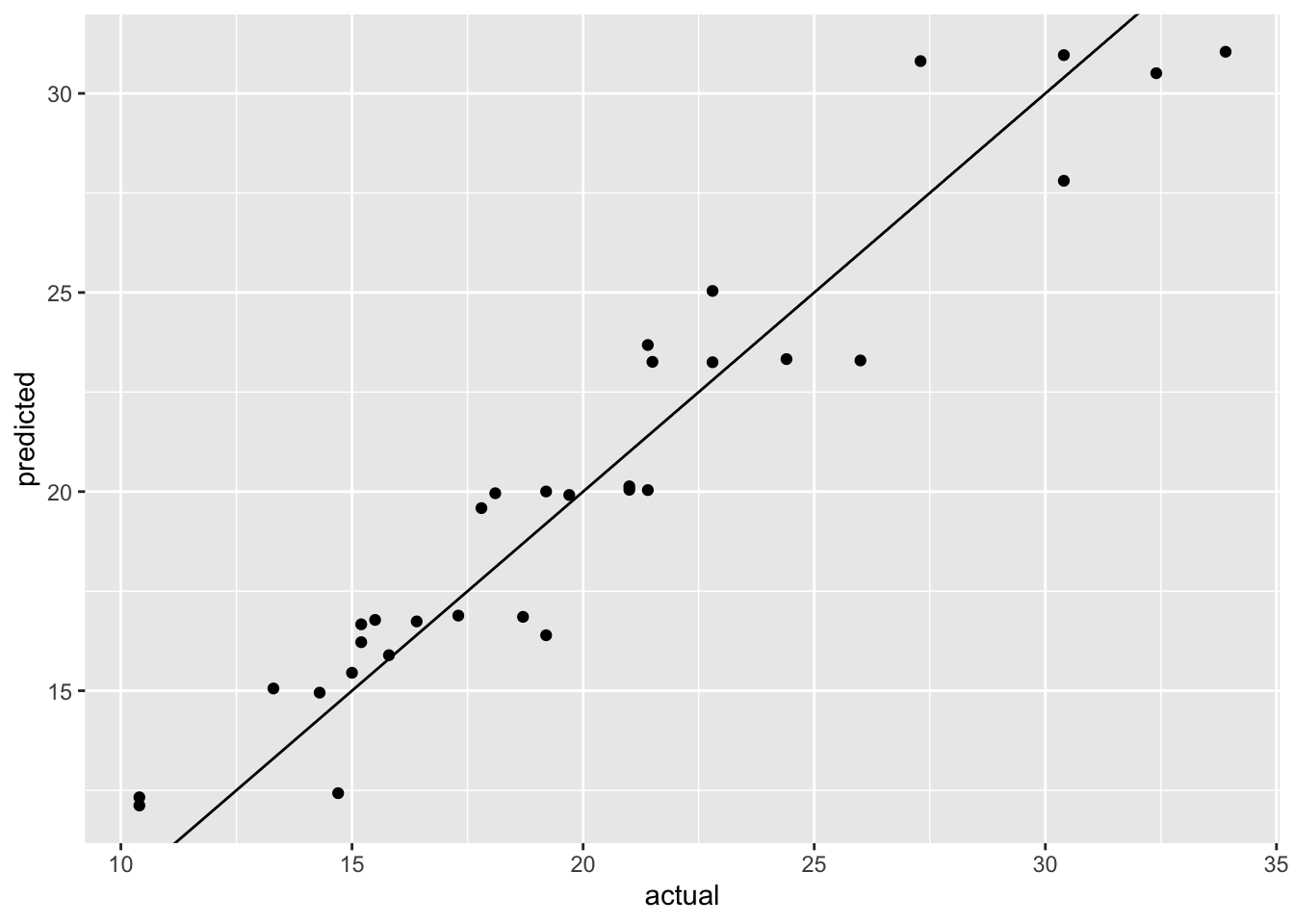

Visualization of actual versus predicted values of mpg — Figure 14.3: Visualization of actual versus predicted values of `mpg`

Figure 14.3 shows the actual versus predicted values for the best model. The model seems to do a good job at predicting the actual values. However, this is the prediction on the training set and we obviously need to assess the model performance on a separate holdout set.

14.4 Grid search strategies

The tune package implements a variety of approaches to search the parameter space.

grid_regular: we used this function in the previous section; it searches the parameter space using a systematic grid of parameter values. In design of experiments, this is known as a full factorial design.
grid_random: this approach randomly samples combinations of parameter values
grid_space_filling: this is a general function that implements different space filling designs to cover the parameter space more evenly. The specific design is specified using the type argument. Use for example:
- default: uses one of several pre-defined space filling designs
- latin_hypercube: Latin hypercube sampling is an approach that comes from the field of experimental design. It is similar to random sampling, but ensures that the parameter space is sampled more evenly.
- max_entropy: maximum entropy sampling also aims to cover the search space evenly.

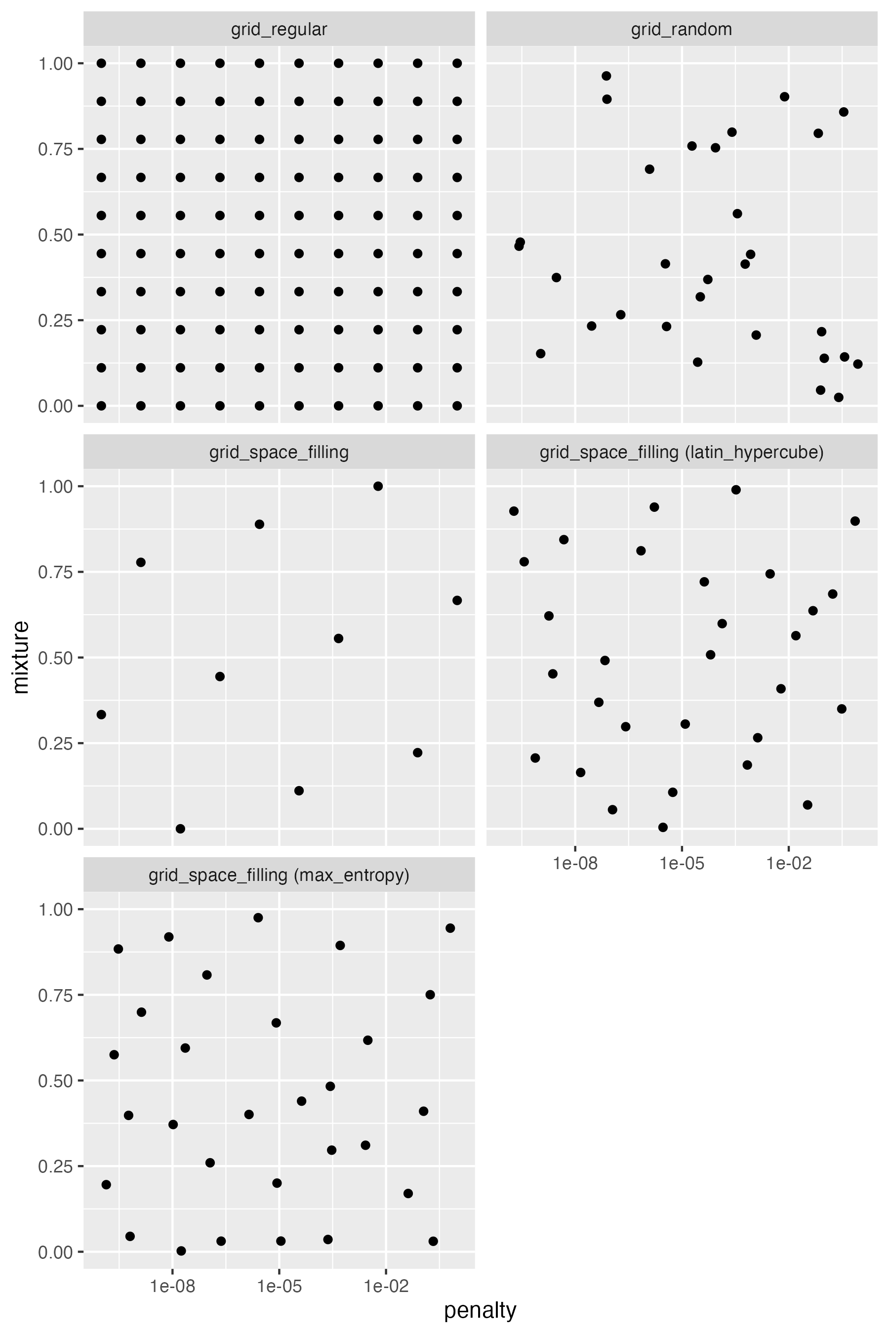
Figure 14.4 shows the difference between the different methods using an example with two continuous parameters, penalty and mixtures, the tuning parameters of a penalized logistic regression model.

The regular grid splits each parameter range into a fixed number of points, here 10, and enumerates all possible combinations of the parameters. This results in 10 x 10 = 100 models. The random grid randomly samples 30 combinations of the parameters. We can see that there are areas of the parameters space that are not well covered. The Latin hypercube and maximum entropy sampling approaches also randomly sample 30 combinations of the parameters, but in this case, there seems to be a more uniform coverage of the parameter space.

Let’s compare the different search strategies using a real example. We will use the mtcars dataset and try to predict the fuel efficiency of cars using a linear regression model. We will use the glmnet engine which allows us to tune L1 and L2 regularization using the penalty and mixture parameters in the linear regression model.

set.seed(123)

recipe <- recipe(mpg ~ ., data = mtcars) %>%
  step_normalize(all_numeric_predictors())
model <- linear_reg(mode = "regression", engine = "glmnet",
  penalty = tune(), mixture = tune())
1wf <- workflow() %>%
  add_recipe(recipe) %>%
  add_model(model)
2parameters <- extract_parameter_set_dials(wf) %>%
  update(
    penalty = penalty(c(-3, 0.75))
  )

1: Define workflow for a regularized linear regression model
2: Define the tuning parameter ranges; defaut values are used for mixture; penalty is adjusted based on preliminary runs (not shown)

We can now apply the different search strategies to tune the model.

1resamples <- vfold_cv(mtcars)
2model_regular <- tune_grid(wf, resamples = resamples,
  grid = grid_regular(parameters, levels = 10))
nrandom <- 30
3model_random <- tune_grid(wf, resamples = resamples,
  grid = grid_random(parameters, size = nrandom))
model_latin_hypercube <- tune_grid(wf, resamples = resamples,
  grid = grid_space_filling(parameters, size = nrandom,
    type = "latin_hypercube"))
model_max_entropy <- tune_grid(wf, resamples = resamples,
  grid = grid_space_filling(parameters, size = nrandom,
    type = "max_entropy"))

1: For better comparison, we use the same resamples for all tuning runs.
2: In this tuning run, we use a regular grid with 10 levels for each parameter, resulting in 100 combinations.
3: This and the following two tuning runs, use random sampling from the parameter space. The first uses random sampling, the second uses a latin hypercube, and the third uses max entropy sampling. All three explore 30 random combinations of the parameters.

df <- rbind(
  cbind(grid = "regular", tested = 100,
    model_regular %>% show_best(metric = "rmse", n = 1)),
  cbind(grid = "random", tested = nrandom,
    model_random %>% show_best(metric = "rmse", n = 1)),
  cbind(grid = "latin_hypercube", tested = nrandom,
    model_latin_hypercube %>% show_best(metric = "rmse", n = 1)),
  cbind(grid = "max_entropy", tested = nrandom,
    model_max_entropy %>% show_best(metric = "rmse", n = 1))
) %>%
  select(-c(.metric, .estimator, n, .config)) %>%
  mutate(
    grid = factor(grid, levels = c(
      "regular", "random", "latin_hypercube", "max_entropy"))
  )

The following table shows the best model for each search strategy.

df %>%
  rename(RMSE = "mean") %>%
  mutate_if(is.numeric, format, digits = 3, nsmall = 0) %>%
  knitr::kable()

grid	tested	penalty	mixture	RMSE	std_err
regular	100	0.825	1.0000	2.48	0.447
random	30	1.654	0.0705	2.51	0.411
latin_hypercube	30	1.851	0.1087	2.52	0.421
max_entropy	30	1.201	0.7782	2.53	0.466

Superficially, it seems that the regular grid search resulted in the best model. However, the difference to the other models is very small and well within the observed variation of the estimated cross-validation performance. Figure 14.5 shows the mean and standard deviation of the RMSE for each search strategy.

ggplot(df, aes(x = grid, y = mean,
    ymin = mean - std_err, ymax = mean + std_err)) +
  geom_point() +
  geom_pointrange() +
  xlab("Method to define grid") + ylab("Mean rmsq error")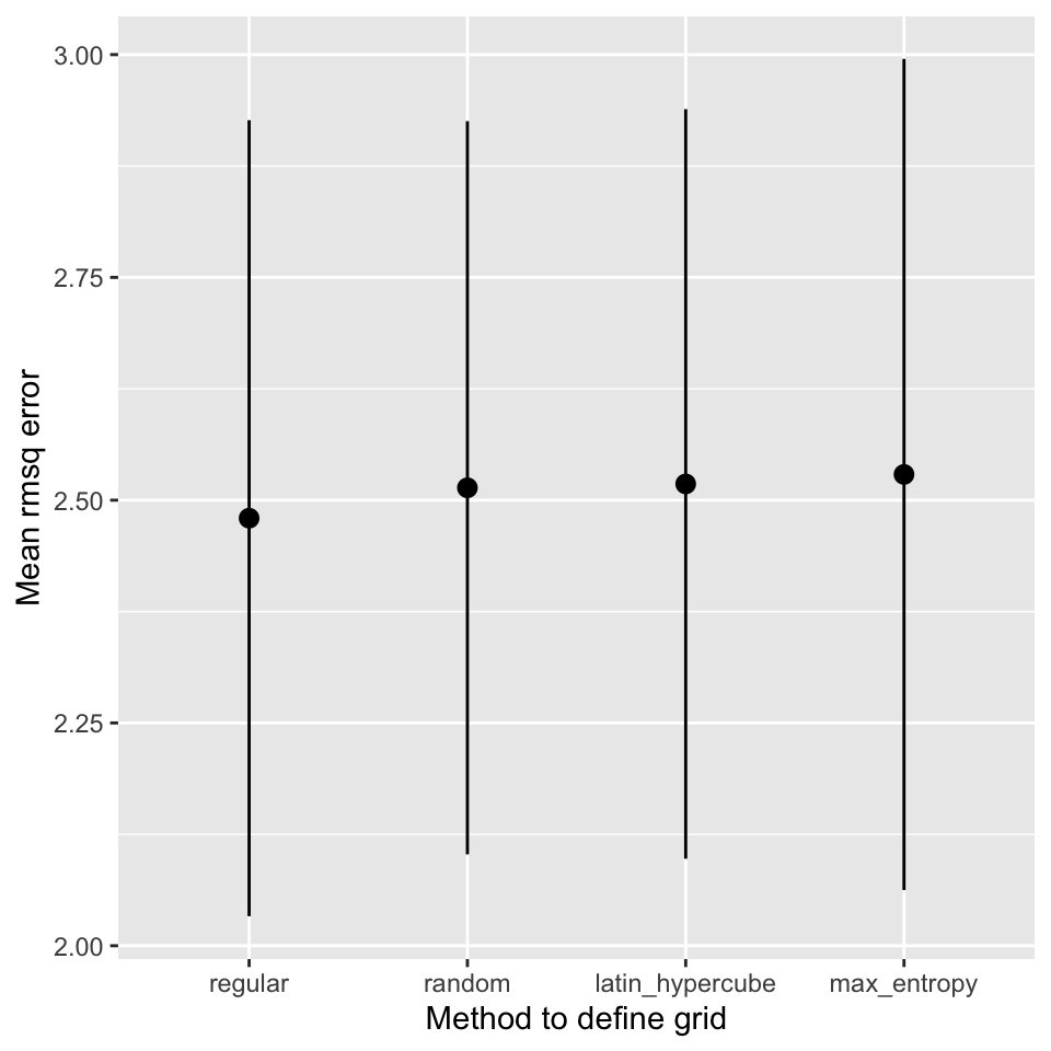

Figure 14.5: Comparison of different search strategies

It is also important to stress, that the regular grid search is much more computationally expensive than the other approaches. The regular grid search tested 100 models, the other methods tested only 30 different models. It also seems as if the best models are obtained for a mixture value of 1, i.e. a pure lasso model. If the best value in the search space is at the boundary of the search space, it is likely that random methods will not find it. If you think this is the case, remove the parameter from tuning and fix the value in the model definition.

Useful to know

In the literature, the regular grid search is usually taught as the default approach to tuning. However, it is not necessarily the best approach. The random approaches are often a better choice. They can be more efficient requiring fewer model evaluations.

14.5 Bayesian Hyperparameter optimization

The tune package also implements Bayesian hyperparameter optimization. Bayesian optimization is a sequential approach to hyperparameter optimization. To initialize the method, random sampling is used to get a rough exploration of the parameter space. Using the validation results, a Bayesian model, a Gaussian process model to be precise, is trained using the parameter combinations as predictors and the validation performance as the outcome. The Gaussian process model then predicts the validation performance for a large number of parameter combinations. This value combined with the uncertainty of the prediction is used to prioritize the next parameter combination finding a trade-off between global exploration and local exploitation. The most useful combination is then evaluated and the process is repeated with the old and new data until a stopping criteria is met (maximum number of iterations or no improvement).

Bayesian hyperparameter optimization is available with the tune_bayes function.

model_bayes <- tune_bayes(wf, resamples = resamples,
  param_info = parameters, iter = 25)

With these settings, the function will create an initial model with 5 evaluations followed by 25 iterations. The param_info argument is used to specify the search space. The iter argument specifies the number of iterations. The tune_bayes function returns a tune_results object that can be used in the same way as the tune_grid function.

Figure 14.6 demonstrates the process of the Bayesian hyperparameter optimization.

regular_metrics <- model_regular %>%
  collect_metrics() %>%
  filter(.metric == "rmse")
bayes_metrics <- model_bayes %>%
  collect_metrics() %>%
  filter(.metric == "rmse")

shapes <- c(
  "Grid search" = 16,
  "Bayesian optimization\n(initial phase)" = 17,
  "Bayesian optimization\n(iterations)" = 15,
  "Bayesian optimization\n(best model)" = 18
)

ggplot(regular_metrics, aes(x = penalty, y = mixture, z = mean)) +
  geom_point(data = df, mapping = aes(shape = "Grid search"),
    color = "red", size = 3) +
  geom_contour(color = "black", alpha = 0.75, bins = 20) +
  geom_point(data = bayes_metrics %>% head(5),
    mapping = aes(shape = "Bayesian optimization\n(initial phase)"),
    size = 3, color = "#6CABBC") +
  geom_point(data = bayes_metrics %>% tail(-5),
    mapping = aes(shape = "Bayesian optimization\n(iterations)"),
    color = "#226DCE") +
  geom_point(
    data = model_bayes %>% show_best(n = 1, metric = "rmse"),
    mapping = aes(shape = "Bayesian optimization\n(best model)"),
    color = "#85db66", size = 3) +
  scale_x_log10() +
  scale_shape_manual(name = "Tuning method", values = shapes)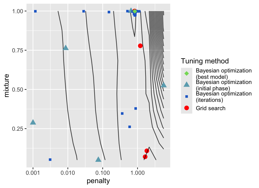

Figure 14.6: Exploration of parameter space during Bayesian hyperparameter tuning for a penalized linear regression model.

The plot shows the parameter combinations that were evaluated during the optimization process. The contour plot was determined from the validation performance calculated for the regular grid search. The blue points show the parameter combinations that were evaluated during the Bayesian hyperparameter optimization. Light blue points were evaluated in the initial phase, the darker blue points were evaluated in the subsequent iterations. The dark blue point highlights the best model found during these iterations. The red point shows the best results from the above grid searches for comparison.

Figure 14.6 clearly shows that the Bayesian hyperparameter optimization fullfills two objectives, exploration by evaluating parameter combinations in areas of the parameter space that have not been explored before and exploitation by evaluating parameter combinations that are close to the best parameter combination found so far.

Further information

https://tune.tidymodels.org/ tune package
https://dials.tidymodels.org/ dials package

There are more packages that extend the capabilities of the tune package.

finetune package implements iterative methods similar to the Bayesian hyperparameter optimization approach, e.g. simulated annealing for global optimization

Code

The code of this chapter is summarized here.

Show the code

knitr::opts_chunk$set(echo = TRUE, cache = TRUE, autodep = TRUE,
  fig.align = "center")
knitr::include_graphics("images/model_workflow_tune.png")
library(tidymodels)
mtcars_rec <- recipe(mpg ~ ., data = mtcars) %>%
  step_normalize(all_numeric_predictors()) %>%
  step_pca(all_numeric_predictors(), num_comp = tune())
model <- nearest_neighbor(mode = "regression", neighbors = tune())
mtcars_workflow <- workflow() %>%
  add_recipe(mtcars_rec) %>%
  add_model(model)
parameters <- extract_parameter_set_dials(mtcars_workflow)
parameters %>% knitr::kable()
parameters$object[1]
parameters$object[2]
parameters <- parameters %>%
  update(
    num_comp = num_comp(c(1, 10)),
    neighbors = neighbors(c(1, 5)),
  )
wf <- workflow() %>%
  add_recipe(mtcars_rec) %>%
  add_model(rand_forest(mtry = tune(), mode = "regression"))
p <- extract_parameter_set_dials(wf)
p
p$object[[1]]
p <- extract_parameter_set_dials(wf) %>%
  finalize(mtcars %>% select(-mpg))
p$object[[1]]
set.seed(123)
tune_results <- tune_grid(mtcars_workflow,
  resamples = vfold_cv(mtcars), grid = grid_regular(parameters))
autoplot(tune_results)
collect_metrics(tune_results) %>% head(7)
show_best(tune_results, metric = "rmse")
best_parameters <- select_best(tune_results, metric = "rmse") %>%
  select(-.config)
best_parameters
best_workflow <- mtcars_workflow %>%
  finalize_workflow(best_parameters) %>%
  fit(mtcars)
best_workflow
df <- tibble(
  actual = mtcars$mpg,
  predicted = predict(best_workflow, new_data = mtcars)$.pred
)

ggplot(df, aes(x = actual, y = predicted)) +
  geom_point() +
  geom_abline()
knitr::include_graphics("images/tuning-grids.png")
set.seed(123)

recipe <- recipe(mpg ~ ., data = mtcars) %>%
  step_normalize(all_numeric_predictors())
model <- linear_reg(mode = "regression", engine = "glmnet",
  penalty = tune(), mixture = tune())
wf <- workflow() %>%
  add_recipe(recipe) %>%
  add_model(model)
parameters <- extract_parameter_set_dials(wf) %>%
  update(
    penalty = penalty(c(-3, 0.75))
  )
resamples <- vfold_cv(mtcars)
model_regular <- tune_grid(wf, resamples = resamples,
  grid = grid_regular(parameters, levels = 10))
nrandom <- 30
model_random <- tune_grid(wf, resamples = resamples,
  grid = grid_random(parameters, size = nrandom))
model_latin_hypercube <- tune_grid(wf, resamples = resamples,
  grid = grid_space_filling(parameters, size = nrandom,
    type = "latin_hypercube"))
model_max_entropy <- tune_grid(wf, resamples = resamples,
  grid = grid_space_filling(parameters, size = nrandom,
    type = "max_entropy"))
df <- rbind(
  cbind(grid = "regular", tested = 100,
    model_regular %>% show_best(metric = "rmse", n = 1)),
  cbind(grid = "random", tested = nrandom,
    model_random %>% show_best(metric = "rmse", n = 1)),
  cbind(grid = "latin_hypercube", tested = nrandom,
    model_latin_hypercube %>% show_best(metric = "rmse", n = 1)),
  cbind(grid = "max_entropy", tested = nrandom,
    model_max_entropy %>% show_best(metric = "rmse", n = 1))
) %>%
  select(-c(.metric, .estimator, n, .config)) %>%
  mutate(
    grid = factor(grid, levels = c(
      "regular", "random", "latin_hypercube", "max_entropy"))
  )
df %>%
  rename(RMSE = "mean") %>%
  mutate_if(is.numeric, format, digits = 3, nsmall = 0) %>%
  knitr::kable()
ggplot(df, aes(x = grid, y = mean,
    ymin = mean - std_err, ymax = mean + std_err)) +
  geom_point() +
  geom_pointrange() +
  xlab("Method to define grid") + ylab("Mean rmsq error")
model_bayes <- tune_bayes(wf, resamples = resamples,
  param_info = parameters, iter = 25)
regular_metrics <- model_regular %>%
  collect_metrics() %>%
  filter(.metric == "rmse")
bayes_metrics <- model_bayes %>%
  collect_metrics() %>%
  filter(.metric == "rmse")

shapes <- c(
  "Grid search" = 16,
  "Bayesian optimization\n(initial phase)" = 17,
  "Bayesian optimization\n(iterations)" = 15,
  "Bayesian optimization\n(best model)" = 18
)

ggplot(regular_metrics, aes(x = penalty, y = mixture, z = mean)) +
  geom_point(data = df, mapping = aes(shape = "Grid search"),
    color = "red", size = 3) +
  geom_contour(color = "black", alpha = 0.75, bins = 20) +
  geom_point(data = bayes_metrics %>% head(5),
    mapping = aes(shape = "Bayesian optimization\n(initial phase)"),
    size = 3, color = "#6CABBC") +
  geom_point(data = bayes_metrics %>% tail(-5),
    mapping = aes(shape = "Bayesian optimization\n(iterations)"),
    color = "#226DCE") +
  geom_point(
    data = model_bayes %>% show_best(n = 1, metric = "rmse"),
    mapping = aes(shape = "Bayesian optimization\n(best model)"),
    color = "#85db66", size = 3) +
  scale_x_log10() +
  scale_shape_manual(name = "Tuning method", values = shapes)

This is not quite true for the number of principal components, however transformation into principal components is usually done only for datasets with a larger number of features.↩︎