DS-6030 Statistical Learning / Copyright © 2023-2024 Peter Gedeck

Chapter 24 Tidymodels vs Scikit-learn

Scikit-learn, like tidymodels, is a framework to define machine learning models and train them. As an open-source project, it has a large community of contributors and users. It is well-documented and has a wide range of algorithms and tools for data preprocessing, model selection, and evaluation. It is the de facto standard for machine learning in Python. Even if models have no direct implementation in scikit-learn, the third-party libraries often implement the scikit-learn API, making them compatible with the framework. xgboost is a popular example for this.

There are many parallels between Tidymodels and scikit-learn; both have a similar approach to model definition and training. You will recognize many of the ideas and concepts from the tidymodels framework in scikit-learn.

Figure 24.1 shows the Python packages mapped onto the modeling workflow of Figure 6.1.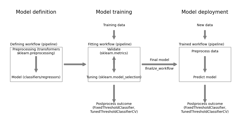

Figure 24.1: Modeling workflow

24.1 Load required packages

Like in R, we start with the import of the required packages:

Code

library(reticulate)
# point reticulate to a Python version with the appropriate packages
use_virtualenv("/Users/petergedeck/git/DS-6030/.venv")

Python:

Code

import pandas as pd
import matplotlib.pyplot as plt
from sklearn import preprocessing
from sklearn.model_selection import (train_test_split, RandomizedSearchCV,
                                     cross_val_predict)
from sklearn.compose import ColumnTransformer
from sklearn.pipeline import Pipeline
from sklearn.linear_model import LogisticRegression

R:

Code

library(tidymodels)

## ── Attaching packages ───────────────────────────────────────────────────────────────────────────────────────────────────────────────── tidymodels 1.2.0 ──

## ✔ broom        1.0.6      ✔ recipes      1.0.10
## ✔ dials        1.2.1      ✔ rsample      1.2.1 
## ✔ dplyr        1.1.4      ✔ tibble       3.2.1 
## ✔ ggplot2      3.5.1      ✔ tidyr        1.3.1 
## ✔ infer        1.0.7      ✔ tune         1.2.1 
## ✔ modeldata    1.3.0      ✔ workflows    1.1.4 
## ✔ parsnip      1.2.1      ✔ workflowsets 1.1.0 
## ✔ purrr        1.0.2      ✔ yardstick    1.3.1

## ── Conflicts ──────────────────────────────────────────────────────────────────────────────────────────────────────────────────── tidymodels_conflicts() ──
## ✖ purrr::discard() masks scales::discard()
## ✖ dplyr::filter()  masks stats::filter()
## ✖ dplyr::lag()     masks stats::lag()
## ✖ recipes::step()  masks stats::step()
## • Use tidymodels_prefer() to resolve common conflicts.

Code

library(tidyverse)

## ── Attaching core tidyverse packages ─────────────────────────────────────────────────────────────────────────────────────────────────── tidyverse 2.0.0 ──
## ✔ forcats   1.0.0     ✔ readr     2.1.5
## ✔ lubridate 1.9.3     ✔ stringr   1.5.1

## ── Conflicts ───────────────────────────────────────────────────────────────────────────────────────────────────────────────────── tidyverse_conflicts() ──
## ✖ readr::col_factor() masks scales::col_factor()
## ✖ purrr::discard()    masks scales::discard()
## ✖ dplyr::filter()     masks stats::filter()
## ✖ stringr::fixed()    masks recipes::fixed()
## ✖ dplyr::lag()        masks stats::lag()
## ✖ readr::spec()       masks yardstick::spec()
## ℹ Use the conflicted package (<http://conflicted.r-lib.org/>) to force all conflicts to become errors

24.2 Load the data

Code

data <- read_csv("https://gedeck.github.io/DS-6030/datasets/loan_prediction.csv",
                 show_col_types=FALSE) %>% 
    drop_na() %>%
    mutate(
        Gender=as.factor(Gender),
        Married=as.factor(Married),
        Dependents=gsub("\\+", "", Dependents) %>% as.numeric(),
        Education=as.factor(Education),
        Self_Employed=as.factor(Self_Employed),
        Credit_History=as.factor(Credit_History),
        Property_Area=as.factor(Property_Area),
        Loan_Status=factor(Loan_Status, levels=c("N", "Y"), labels=c("No", "Yes"))
    ) %>% 
    select(-Loan_ID)

Code

data = pd.read_csv("https://gedeck.github.io/DS-6030/datasets/loan_prediction.csv")
data = data.dropna()
data['Dependents'] = [int(str(s).strip('+')) for s in data['Dependents']]
data['Loan_Status'] = [1 if s == 'Y' else 0 for s in data['Loan_Status']]

outcome = 'Loan_Status'
predictors = ['Gender', 'Married', 'Dependents', 'Education', 'Self_Employed',
              'ApplicantIncome', 'CoapplicantIncome', 'LoanAmount', 'Loan_Amount_Term',
              'Credit_History', 'Property_Area']

24.3 Split the data into training and holdout data

Split dataset into training and holdout data

Code

set.seed(123)
data_split <- initial_split(data, prop=0.8, strata=Loan_Status)
train_data <- training(data_split)
holdout_data <- testing(data_split)

Code

Xtrain, Xholdout, ytrain, yholdout = train_test_split(data[predictors], data[outcome], 
                                                test_size=0.2, random_state=123,
                                                stratify=data[outcome])
Xtrain.shape, Xholdout.shape, ytrain.shape, yholdout.shape

## ((384, 11), (96, 11), (384,), (96,))

24.4 Define the model

R:

Code

formula <- Loan_Status ~ Gender + Married + Dependents + Education + Self_Employed +
           ApplicantIncome + CoapplicantIncome + LoanAmount + Loan_Amount_Term + 
           Credit_History + Property_Area
recipe_spec <- recipe(formula, data=train_data) %>%
    step_dummy(all_nominal(), -all_outcomes())
# recipe_spec %>% prep() %>% bake(new_data=NULL) %>% head()

model_spec <- logistic_reg(engine="glmnet", mode="classification",
                           penalty=tune(), mixture=0)

wf <- workflow() %>%
    add_model(model_spec) %>%
    add_recipe(recipe_spec)

Python:

Code

preprocess = ColumnTransformer([
    ('encoder', preprocessing.OneHotEncoder(drop='first'), 
        ['Gender', 'Married', 'Education', 'Self_Employed', 'Property_Area']),
    ('unchanged', 'passthrough', 
        ['Dependents', 'ApplicantIncome', 'CoapplicantIncome', 'LoanAmount', 
         'Loan_Amount_Term', 'Credit_History']),
])
# preprocess.fit_transform(data).round(4)[:20,]

model = Pipeline([
    ('preprocess', preprocess),
    ('classifier', LogisticRegression(penalty='l2', max_iter=10_000))
])

24.5 Parameter tuning using cross-validation

Code

resamples <- vfold_cv(train_data, v=10, strata=Loan_Status)
cv_metrics <- metric_set(roc_auc, accuracy)
cv_control <- control_resamples(save_pred=TRUE)

Tune the penalty hyperparameter using Bayesian hyperparameter optimization:

Code

parameters <- extract_parameter_set_dials(wf) %>% 
    update(penalty=penalty(c(-3, 0)))
tune_wf <- tune_bayes(wf, resamples=resamples, metrics=cv_metrics,
                      param_info=parameters, iter=25)

## ! No improvement for 10 iterations; returning current results.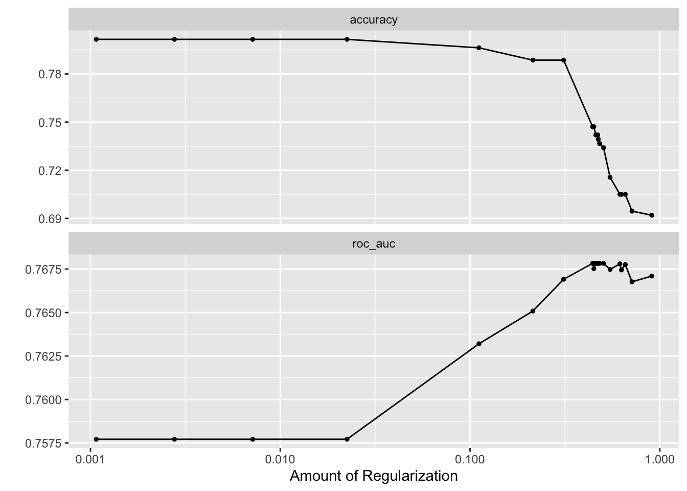

Code

autoplot(tune_wf)

Figure 24.2: Autoplot shows the ROC-AUC for different values of the penalty hyperparameter.

Code

from scipy.stats import loguniform, uniform
hyperparameters = {
    'classifier__C': loguniform(1e-2, 10),
}

clf = RandomizedSearchCV(model, hyperparameters, random_state=0,
                         cv=10, 
                         n_iter=50, scoring='roc_auc', n_jobs=8)
search = clf.fit(Xtrain, ytrain)
search.best_score_, search.best_params_

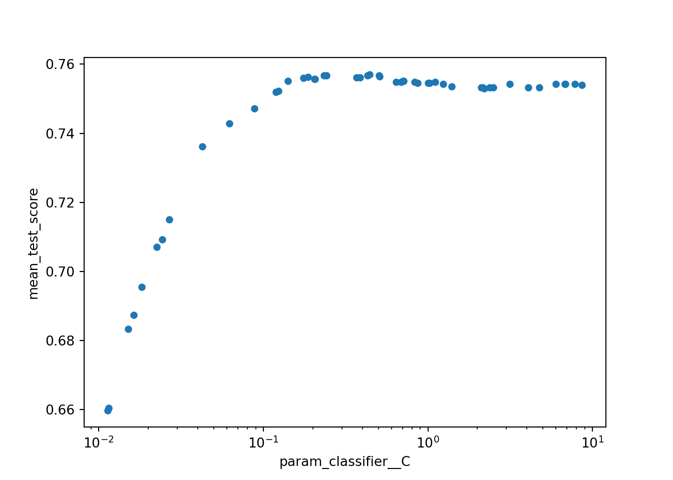
## (np.float64(0.7570491237157904), {'classifier__C': np.float64(0.44303752452182665)})

Code

ax = pd.DataFrame(search.cv_results_).plot.scatter(x='param_classifier__C', 
                                              y='mean_test_score')
ax.set_xscale('log')

24.6 ROC curves

Code

best_parameter <- select_best(tune_wf, metric="roc_auc")
best_wf <- finalize_workflow(wf, best_parameter)
result_cv <-  fit_resamples(best_wf, resamples,
                            metrics=cv_metrics, control=cv_control)

roc_cv_plot <- function(model_cv, model_name) {
  cv_predictions <- collect_predictions(model_cv)
  cv_ROC <- cv_predictions %>% roc_curve(truth=Loan_Status, .pred_Yes, event_level="second")
  autoplot(cv_ROC) +
    labs(title=model_name)
}
roc_cv_plot(result_cv, "Logistic regression")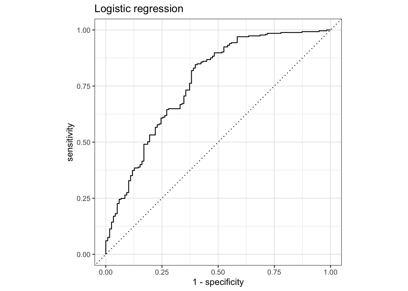

Code

from sklearn.metrics import roc_curve, auc
y_train_pred = cross_val_predict(search.best_estimator_, Xtrain, ytrain, 
                                 cv=10, method='predict_proba')
fpr, tpr, _ = roc_curve(ytrain, y_train_pred[:, 1])

roc_auc = auc(fpr, tpr)

fig, ax = plt.subplots(figsize=[5, 5])
_ = ax.plot(fpr, tpr, color='darkorange',
         lw=2, label=f'ROC curve (area = {roc_auc:0.4f})')
_ = ax.plot([0, 1], [0, 1], color='navy', lw=2, linestyle='--')
_ = ax.set_xlim([0.0, 1.0])
_ = ax.set_ylim([0.0, 1.05])
_ = ax.set_xlabel('False Positive Rate (1 - Specificity)')
_ = ax.set_ylabel('True Positive Rate (Sensitivity)')
_ = ax.legend(loc="lower right")
_ = plt.show()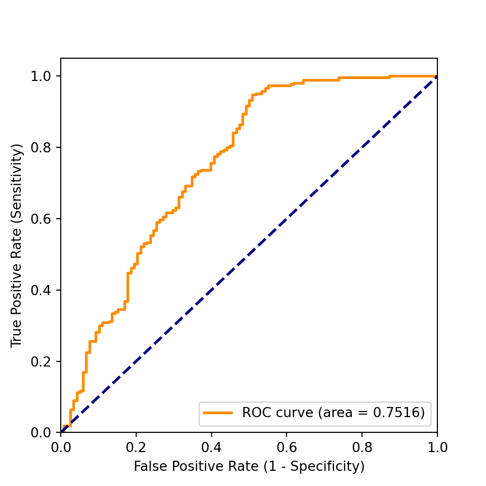

24.7 Finalize the workflow:

Code

best_parameter <- select_best(tune_wf, metric="roc_auc")
best_wf <- finalize_workflow(wf, best_parameter)

The best roc_auc is obtained with a penalty of best_parameter['penalty'] = 0.4738658.

Use the tuned workflow for cross-validation and training the final model using the full dataset:

Code

result_cv <-  fit_resamples(best_wf, resamples,
                            metrics=cv_metrics, control=cv_control)
fitted_model <- best_wf %>% fit(train_data)

Estimate model performance using the cross-validation results and the holdout data:

Code

cv_results <- collect_metrics(result_cv) %>%
    select(.metric, mean) %>%
    rename(.estimate=mean) %>%
    mutate(result="Cross-validation")
holdout_predictions <- augment(fitted_model, new_data=holdout_data)
holdout_results <-  bind_rows(
        c(roc_auc(holdout_predictions, Loan_Status, .pred_Yes, event_level="second")),
        c(accuracy(holdout_predictions, Loan_Status, .pred_class))
    ) %>%
    select(-.estimator) %>%
    mutate(result="Holdout") 

The performance metrics are summarized in the following table.

Code

bind_rows(
    cv_results,
    holdout_results
) %>% 
    pivot_wider(names_from=.metric, values_from=.estimate) %>%
    kableExtra::kbl(caption="Model performance metrics", digits=3) %>%
    kableExtra::kable_styling(full_width=FALSE)

Table 6.1: Model performance metrics

result	accuracy	roc_auc
Cross-validation	0.734	0.768
Holdout	0.763	0.723

Python - By default, scikit_learn determines and returns the “best model” after cross-validation.

Code

from sklearn import metrics
best_model = search.best_estimator_
y_holdout_pred = best_model.predict(Xholdout)

pd.DataFrame({
    'Accuracy': [
        metrics.accuracy_score(ytrain, [1 if p > 0.5 else 0 for p in y_train_pred[:, 1]]),
        metrics.accuracy_score(yholdout, y_holdout_pred)],
    'ROC AUC': [
        metrics.roc_auc_score(ytrain, y_train_pred[:, 1]),
        metrics.roc_auc_score(yholdout, best_model.predict_proba(Xholdout)[:, 1])
    ],
}, index=['Cross-validation', 'Testset'])

##                   Accuracy   ROC AUC
## Cross-validation  0.809896  0.751593
## Testset           0.781250  0.715657