Chapter 28 Markdown

In Markdown, the code is executed and the results are included in the document. This is a very powerful way of writing a document. If you change the code, the document is updated automatically. This is very useful if you need to update a document regularly. For example, if you need to update a report every month with the latest data. For larger documents that require considerable computation time, caching can be used to speed up the process (see Appendix 27.2).

28.1 General syntax

See https://www.rstudio.com/wp-content/uploads/2015/03/rmarkdown-reference.pdf for an overview of the Markdown syntax.

28.2 Code chunks

In order to embed R code in a document, we use the following syntax:

```{r chunk-name}
x = 123
```

The three backticks define a code block. The {r} indicates that we want to execute the content using R. Here, we also name the code chunk chunk-name. This is optional but useful, and required if you want to use caching (see 27.2) or reference figures.

28.3 Chunk options

There are many options to control the behavior of a code chunk. In this document, we used a subset of them. Use the following to avoid displaying warnings and messages:

```{r chunk-name}
#| warning: FALSE
#| message: FALSE
...
```

However, only add these options if you understand what the displayed warning or message means and you are sure that you want to hide it.

28.4 Figures

Figures come with a large number of options. The ones we used in this document are:

fig.cap: Caption of the figure.
fig.width: Width of the figure in inches.
fig.height: Height of the figure in inches.
fig.align: Alignment of the figure. Possible values are left, right and center.
dev: Specifies the format of the figure. The default depends on the output format. For HTML, the default is png; for PDF it is pdf. If you create a PDF file and your graph contains a large number of points, it will be better to use #| dev: png to avoid a large file size and faster rendering of the PDF.

```{r figure-demo}
#| fig.cap: "Figure caption shown below the plot"
#| fig.width: 4
#| fig.height: 4
#| fig.align: "center"
#| out.width: 75%
#| dev: "png"
plot(1:10)
```

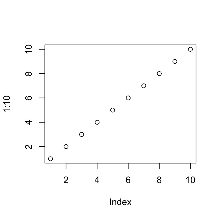
This will create the following table with the caption shown below the plot. The width of the figure is 75% of the text width and figure is centered.

Figure 28.1: Figure caption shown below the plot

In markdown, we can reference the Figure using \@ref(fig:figure-demo). For example, Figure 28.1 shows a plot of the numbers 1 to 10.

If your references don’t show up, check if you knit to either bookdown::pdf_document2 or bookdown::html_document2. The previous format for HTML documents (html_document) requires a different format for references.

Currently, knitting to PDF using markdown requires to have either out.width or fig.align specified. Otherwise, the resulting document will neither contain a figure caption nor will references work. You can also set fig.align as a global option:

knitr::opts_chunk$set(fig.align="center")

28.5 Referencing R variables in text

Sometimes, you might want to reference calculation results in your text. If you add the results manually, but later on change the calculations, the actual results and the text will no longer reference the same values. It is possible to embed results in text using markdown to avoid this situation. Here is an example:

Code

rmse <- 1.2345678

We can reference the variable rmse in the text using:

The RMSE value is `r round(rmse, 3)`.

The command round(rmse, 3) will be executed and the result shown in the text:

The RMSE value is 1.235.

Further information:

Overview of R markdown options: https://www.rstudio.com/wp-content/uploads/2015/03/rmarkdown-reference.pdf