Chapter 22 Generalized additive models (GAM)
In linear regression, the outcome is a linear function of the predictor variables. \[ y = y_0 + c_1 x_1 + c_2 x_2 + c_3 x_3 + \dots \] where \(c_i\) are the coefficients and \(y_0\) is the intercept.
Generalized linear models (GLMs) extend this idea by adding a link function to the outcome variable. \[ g(y) = y_0 + c_1 x_1 + c_2 x_2 + c_3 x_3 + \dots \] Here, \(g\) is the link function. The normal linear regression model uses the identity function \(g(x) = x\). For logistic regression, the link function is \(g(x) = \ln\frac{x}{1-x}\).
A generalized additive model (GAM) extends the concept even further and describes the outcome as a linear function of transformed predictor variables. \[ g(y) = y_0 + c_1 f_1(x_1) + c_2 f_2(x_2) + c_3 f_3(x_3) + \dots \] The functions \(f_i\) are usually smooth functions, such as splines, that are estimated from the data. The coefficients \(c_i\) are estimated using maximum likelihood estimation.
GAMs are useful when the relationship between the outcome and the predictor variables is not linear. For example, the relationship may be quadratic or sinusoidal. GAMs are also useful when the relationship is not known in advance and will be estimated from the data.
22.1 Specifying GAMs in formula notation
The GAM models extend the formula notation with special smoothing terms. Here is an example:
mpg ~ s(displacement) + s(horsepower) + s(weight) + acceleration + yearThe s() function indicates that the variable is smoothed. The smoothing is done using splines. See the documentation for full details.
22.2 GAMs in Tidymodels
In tidymodels, GAMs are available with the gen_additive_mod function from the parsnip package. The only available engine that can be used is the mgcv packge. The next section will demonstrate how to train GAM models in tidymodels. However, workflows requires a different approach from what we’ve seen so far.
22.3 Example: GAM for the mpg dataset
In the following, we use the ISLR2::Auto dataset to predict the fuel efficiency of cars. Load and preprocess the data:
Code
The dataset contains 392 observations with 8 variables. The outcome variable is mpg and the predictor variables are displacement, horsepower, weight, acceleration, and year.
22.3.1 Utility functions
For convenience, we define a series of utility functions. Open the code block to see the implementations.
Code
# create a residual plot
residual_plot <- function(model_fit, data, outcome) {
result <- tibble(prediction = predict(model_fit, new_data=data)$.pred)
result["residual"] <- data[outcome] - result["prediction"]
g <- ggplot(result, aes(x=prediction, y=residual)) +
geom_point() +
geom_hline(yintercept=0, linetype="dashed") +
geom_smooth(method="loess", formula = "y ~ x") +
labs(x="Predicted mpg", y="Residuals")
return(g)
}
# collect and show model metrics
append_model_metrics <- function(model_metrics, model_fit, model_name) {
model_metrics <- bind_rows(
model_metrics,
bind_cols(
model=model_name,
metrics(augment(model_fit, new_data=auto), truth=mpg, estimate=.pred)
)
)
return(model_metrics)
}
show_metrics_table <- function(model_metrics) {
model_metrics %>%
pivot_wider(names_from=.metric, values_from=.estimate) %>%
select(-.estimator) %>%
knitr::kable(digits=3) %>%
kableExtra::kable_styling(full_width=FALSE)
}22.3.2 Linear regression model
Code
| model | rmse | rsq | mae |
|---|---|---|---|
| Linear model | 3.409 | 0.809 | 2.619 |
The residual plot is shown in Figure 22.1.
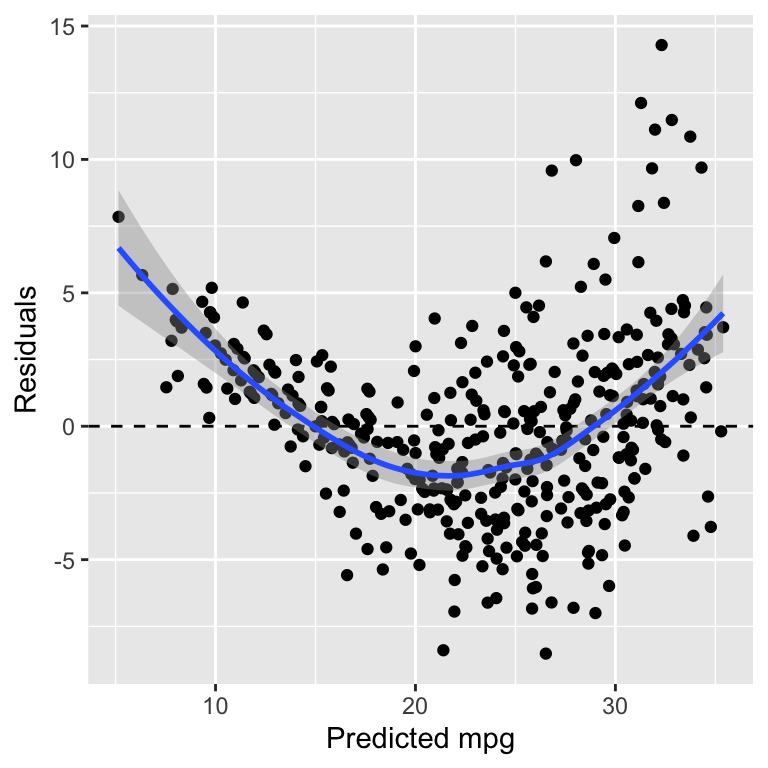
Figure 22.1: Residuals of the linear regression model
We observe two issues with the residuals vs. fit plot.
- The residuals are fanning out, i.e. they have a small spread for small values of the predicted mpg and a larger spread for larger values of the predicted mpg.
- The graph shows a non-linear relationship
Both observations indicate that the model is not a good fit for the data. An obvious approach would be to add quadratic terms to the model. GAMs are an alternative way of addressing this issue.
22.3.3 GAM with splines
We start by adding smoothers to the variable displacement, horsepower, weight, and acceleration.
Code
gam_formula <- mpg ~ s(displacement) + s(horsepower) + s(weight) + s(acceleration) + year
gam_model <- gen_additive_mod() %>%
set_engine("mgcv") %>%
set_mode("regression") %>%
fit(gam_formula, data=auto)
model_metrics <- append_model_metrics(model_metrics, gam_model, "GAM")
show_metrics_table(model_metrics)| model | rmse | rsq | mae |
|---|---|---|---|
| Linear model | 3.409 | 0.809 | 2.619 |
| GAM | 2.835 | 0.868 | 2.084 |
The metrics show that the GAM model is a much better fit than the linear regression model. This is also obvious in the residual plot in Figure 22.2. The residuals are smaller and the non-linearity is less pronounced.
Code
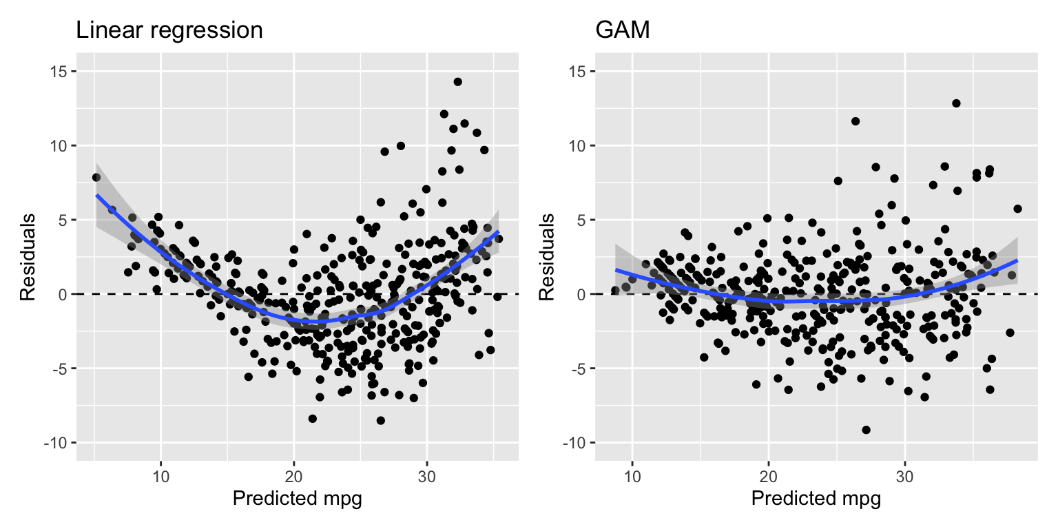
Figure 22.2: Residuals of the linear regression (left) and GAM (right) models
There is still some heteroskedasticity in the residuals.
22.3.4 GAM in workflows
The GAM model can also be used in a workflow. However, we can only use formulas in recipes that specify variables and not transformations. Instead, we need to use the add_variables method and specify the formula in the add_model function.
Code
spec <- gen_additive_mod() %>%
set_engine("mgcv") %>%
set_mode("regression")
wf <- workflow() %>%
add_variables(outcomes = c(mpg),
predictors = c(displacement, horsepower, weight, acceleration, year)) %>%
add_model(spec, formula = gam_formula)
wf_model <- wf %>% fit(data = auto)
model_metrics <- append_model_metrics(model_metrics, wf_model, "GAM-wf")
show_metrics_table(model_metrics)| model | rmse | rsq | mae |
|---|---|---|---|
| Linear model | 3.409 | 0.809 | 2.619 |
| GAM | 2.835 | 0.868 | 2.084 |
| GAM-wf | 2.835 | 0.868 | 2.084 |
The metrics are, as expected, identical to the results from the previous GAM model and Figure 22.3 shows the same residual plot as before.
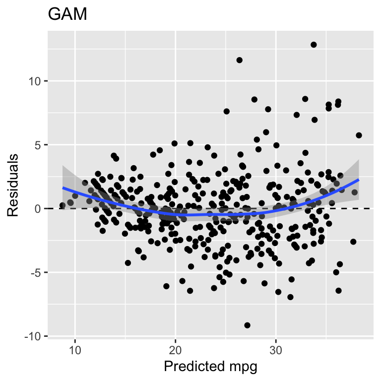
Figure 22.3: Residuals of the linear regression model trained using a workflow
However, using a workflow, we can also use a recipe and specify transformations to the variables. For example, we can use the Yeo-Johnson transformation to transform the variables as shown in the following example.
Code
rec <- recipe(mpg ~ displacement + horsepower + weight + acceleration + year, data=auto) %>%
step_YeoJohnson(all_numeric_predictors())
spec <- gen_additive_mod() %>%
set_engine("mgcv") %>%
set_mode("regression")
wf <- workflow() %>%
add_recipe(rec) %>%
add_model(spec, formula = gam_formula)
wf_model_2 <- wf %>% fit(data = auto)
model_metrics <- append_model_metrics(model_metrics, wf_model_2, "GAM-wf-2")
show_metrics_table(model_metrics)| model | rmse | rsq | mae |
|---|---|---|---|
| Linear model | 3.409 | 0.809 | 2.619 |
| GAM | 2.835 | 0.868 | 2.084 |
| GAM-wf | 2.835 | 0.868 | 2.084 |
| GAM-wf-2 | 2.800 | 0.871 | 2.075 |
The performance metrics are slightly better than before and if you analyze the residual plot, there is a hint of a reduction in the heteroskedasticity. Note however that the formula now refers to the transformed variables and not the original variables.
22.4 Using the plot function of the mgcv model
The mgcv package provides a plot function that can be used to visualize the components of the GAM model. The following code block shows how to use this function. It is important to explicitly load the mgcv package. Otherwise, the plot function will not be available. Note the argument scale=0 which ensures that the plots are not scaled to the same y-axis. This is useful to see the individual components of the model.
Code
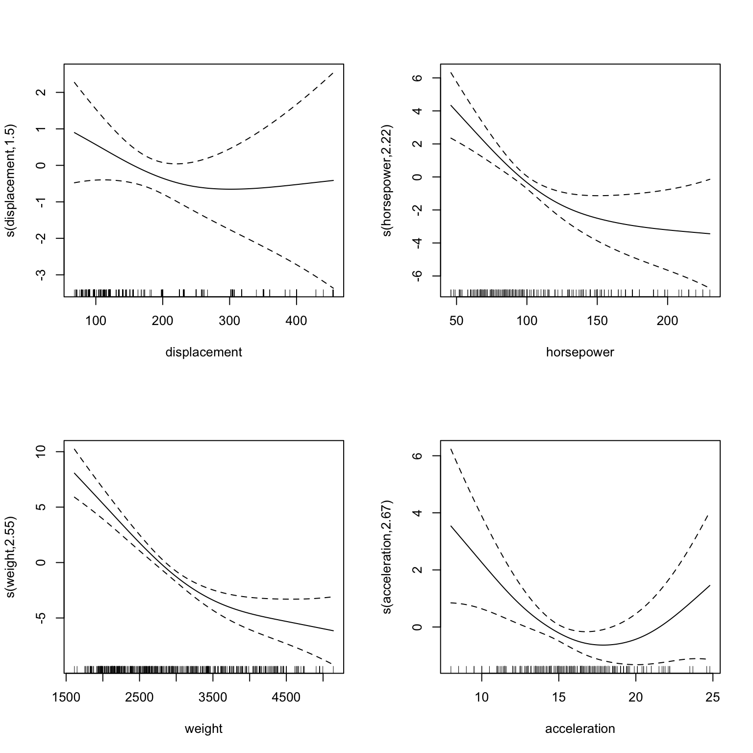
Figure 22.4: Plots of the GAM model
Figure 22.4 shows that the GAM model fits spline with for displacement and horsepower with considerable non-linearity.
We can also visualize the components from the workflow model. Figure 22.5 shows the results. As already mentioned, the formula refers to the transformed variables, so displacment now refers to the Yeo-Johnson transformed variable. Note, the more evenly distributed data points in the rug plot components.
Code
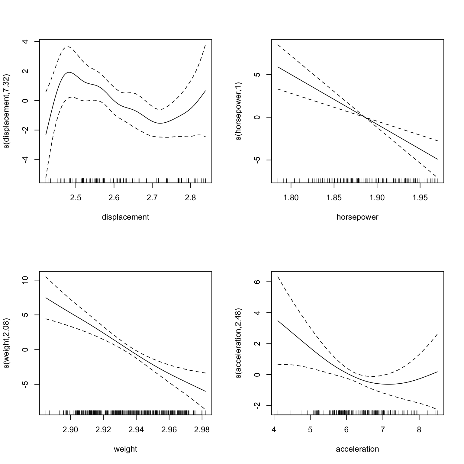
Figure 22.5: Plots of the GAM model
Further information:
Code
The code of this chapter is summarized here.
Code
knitr::opts_chunk$set(echo=TRUE, cache=TRUE, autodep=TRUE, fig.align="center")
library(tidymodels)
library(tidyverse)
library(patchwork)
auto <- ISLR2::Auto %>%
    as_tibble() %>%
    mutate(
        cylinders=as.factor(cylinders),
        origin=as.factor(origin),
    ) %>%
    select(-name)
# create a residual plot
residual_plot <- function(model_fit, data, outcome) {
    result <- tibble(prediction = predict(model_fit, new_data=data)$.pred)
    result["residual"] <- data[outcome] - result["prediction"]
    g <- ggplot(result, aes(x=prediction, y=residual)) +
        geom_point() +
        geom_hline(yintercept=0, linetype="dashed") +
        geom_smooth(method="loess", formula = "y ~ x") +
        labs(x="Predicted mpg", y="Residuals")
    return(g)
}

# collect and show model metrics
append_model_metrics <- function(model_metrics, model_fit, model_name) {
    model_metrics <- bind_rows(
        model_metrics,
        bind_cols(
            model=model_name,
            metrics(augment(model_fit, new_data=auto), truth=mpg, estimate=.pred)
        )
    )
    return(model_metrics)
}

show_metrics_table <- function(model_metrics) {
    model_metrics %>%
        pivot_wider(names_from=.metric, values_from=.estimate) %>%
        select(-.estimator) %>%
        knitr::kable(digits=3) %>%
        kableExtra::kable_styling(full_width=FALSE)
}
formula <- mpg ~ displacement + horsepower + weight + acceleration + year
lm_model <- linear_reg() %>%
    set_engine("lm") %>%
    fit(formula, data=auto)
model_metrics <- append_model_metrics(tibble(), lm_model, "Linear model")
show_metrics_table(model_metrics)
residual_plot(lm_model, auto, "mpg")
gam_formula <- mpg ~ s(displacement) + s(horsepower) + s(weight) + s(acceleration) + year
gam_model <- gen_additive_mod() %>%
    set_engine("mgcv") %>%
    set_mode("regression") %>%
    fit(gam_formula, data=auto)

model_metrics <- append_model_metrics(model_metrics, gam_model, "GAM")
show_metrics_table(model_metrics)
g1 <- residual_plot(lm_model, auto, "mpg") +
    labs(title="Linear regression") +
    ylim(-10, 15)
g2 <- residual_plot(gam_model, auto, "mpg") +
    labs(title="GAM") +
    ylim(-10, 15)
g1 + g2
spec <- gen_additive_mod() %>%
    set_engine("mgcv") %>%
    set_mode("regression")

wf <- workflow() %>%
    add_variables(outcomes = c(mpg),
        predictors = c(displacement, horsepower, weight, acceleration, year)) %>%
    add_model(spec, formula = gam_formula)
wf_model <- wf %>% fit(data = auto)
model_metrics <- append_model_metrics(model_metrics, wf_model, "GAM-wf")
show_metrics_table(model_metrics)
residual_plot(wf_model, auto, "mpg") +
    labs(title="GAM")
rec <- recipe(mpg ~ displacement + horsepower + weight + acceleration + year, data=auto) %>%
    step_YeoJohnson(all_numeric_predictors())
spec <- gen_additive_mod() %>%
    set_engine("mgcv") %>%
    set_mode("regression")

wf <- workflow() %>%
    add_recipe(rec) %>%
    add_model(spec, formula = gam_formula)
wf_model_2 <- wf %>% fit(data = auto)
model_metrics <- append_model_metrics(model_metrics, wf_model_2, "GAM-wf-2")
show_metrics_table(model_metrics)
library(mgcv)  # this is important to load the plot function
opar <- par(mfrow=c(2, 2))
plot(gam_model %>% extract_fit_engine(), scale=0)
par(opar)
library(mgcv)  # this is important to load the plot function
opar <- par(mfrow=c(2, 2))
plot(wf_model_2 %>% extract_fit_engine(), scale=0)
par(opar)