Chapter 24 Variable or feature importance
variable importance, also known as feature importance, is a measure of the influence of a feature on the prediction of a model. It helps you understand why a model makes a specific prediction and explain it. It can also help you to identify potential bias and errors in the model.
The approaches to calculate variable importance can be grouped into local and global measures of variable importance. Local measures are calculated for a single prediction, while global measures are calculated for the entire dataset.
In this chapter, we will focus on global measures of variable importance. We will use the vip package to calculate variable importance for a random forest model trained on the mtcars dataset. The vip package provides a unified interface to calculate variable importance for different models and datasets. It supports different methods to calculate variable importance, such as permutation-based importance, SHAP values, and others.
Load required libraries
Code
24.1 The vip package
The vip package provides a unified interface to calculate variable importance for different models and datasets.
24.2 Model specific measures of variable importance
24.2.1 Linear model
A common measure of variable importance in linear models is the \(t\)-statistic.
Let’s start with a linear regression model trained on the mtcars dataset to predict mpg.
Code
To use the vip package, we need to extract the fit engine from the workflow and pass it to the vip function. Figure 24.1 shows the resulting graph:
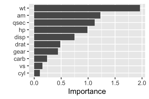
Figure 24.1: Variable importance for a linear regression model (t-statistic)
If we compare the graph with the coefficients of the linear model, we see that the graph shows the absolute values of the \(t\)-statistic of the coefficients.
## Estimate Std. Error t value Pr(>|t|)
## (Intercept) 20.0906250 0.4684931 42.8835050 6.185024e-22
## cyl -0.1990240 1.8663298 -0.1066392 9.160874e-01
## disp 1.6527522 2.2132353 0.7467585 4.634887e-01
## hp -1.4728757 1.4925162 -0.9868407 3.349553e-01
## drat 0.4208515 0.8743992 0.4813036 6.352779e-01
## wt -3.6352668 1.8536038 -1.9611887 6.325215e-02
## qsec 1.4671532 1.3059782 1.1234133 2.739413e-01
## vs 0.1601576 1.0607063 0.1509915 8.814235e-01
## am 1.2575703 1.0262499 1.2254035 2.339897e-01
## gear 0.4835664 1.1017333 0.4389142 6.652064e-01
## carb -0.3221020 1.3386010 -0.2406258 8.121787e-01The most influentials features are, unsurprisingly, wt, am, qsec, and hp.
24.2.2 Random forests
Let’s begin with training a random forest model using the ranger package. By setting the importance argument, the ranger model will collect information about the effect of each feature on improving the model’s performance at each split in the decision trees.
Code
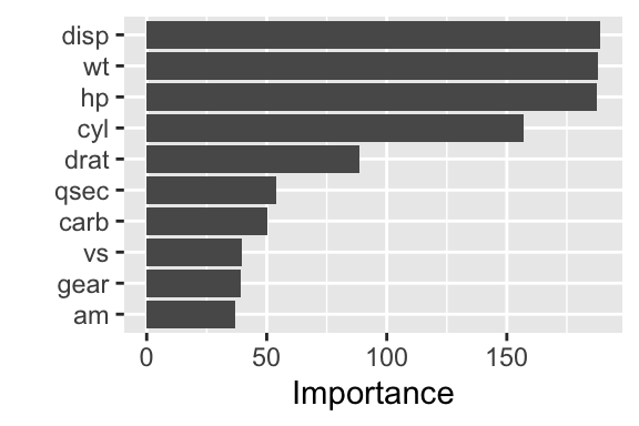
Figure 24.2: Variable importance for a linear regression model (random forest)
The result is shown in Figure 24.2. This time, different features are considered most important: disp, wt, hp, and cyl.
24.3 General approaches to calculate variable importance
While the model-specific measures of variable importance are useful, more general approaches were developed to determine variable importance for a wider range of models.
Figure 24.3 shows the variable importance calculated using the FIRM method (left) and the permutation method (right).
Code
# extract the RF model from the workflow
rf_model <- rf_fit %>% extract_fit_engine()
# Define a prediction wrapper function
pfun <- function(object, newdata) {
predict(object, data = newdata)$predictions
}
vis_firm <- vi(rf_model, method="firm", target="mpg", metric="rmse",
pred_wrapper=pfun, train=bake(prep(mtcars_rec), new_data=NULL))
g1 <- vip(vis_firm) + labs(title="FIRM")
vis_permute <- vi(rf_model, method="permute", target="mpg", metric="rmse",
nsim=10, pred_wrapper=pfun, train=bake(prep(mtcars_rec), new_data=NULL))
g2 <- vip(vis_permute) + labs(title="Permutation")
g1 + g2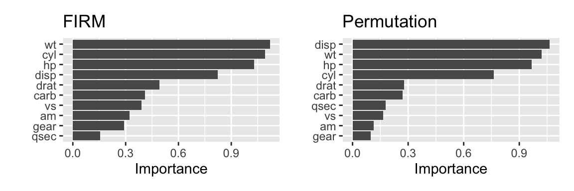
Figure 24.3: Variable importance determined using FIRM (left) and permutation approach (right)
The FIRM method looks at the effect of each feature on the prediction of the model. It is based on partial dependency plots. The effect of each predictor is determined by measuring the variation in the model’s prediction when the feature is changed while keeping all other features constant. Figure 24.4 shows the partial dependency plots for each feature. The individual graphs are ordered in decreasing importance according to the FIRM method.
Code
# combine effects into a single data frame
effects <- attr(vis_firm, which = "effects")
effect_data <- tibble()
for (name in vis_firm$Variable) {
effect <- effects[[name]]
effect_data <- effect_data %>%
bind_rows(tibble(name=name, predictor=effect[[name]], yhat=effect$yhat))
}
# order the predictors by FIRM importance
effect_data <- effect_data %>%
mutate(name=factor(name, levels=vis_firm$Variable))
ggplot(effect_data, aes(x=predictor, y=yhat)) +
geom_line() +
facet_wrap(~name, ncol=5)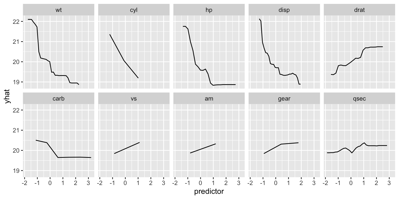
Figure 24.4: Partial dependency plots for each feature
The permutation method is a more straightforward approach. It calculates the variable importance by permuting the values of each feature and measuring the change in the model’s performance. In our calculation of vis_permute we used nsim=10 permutations. The individual results are shown in Figure 24.5.
Code
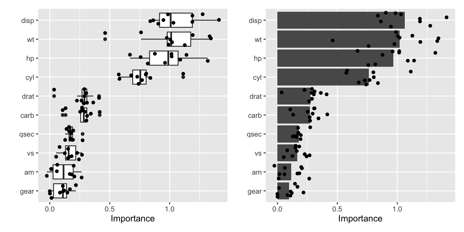
Figure 24.5: Different visualizations of the results of the permutation method
Further information: Additional information can be found in the following resources:
Code
The code of this chapter is summarized here.
Code
knitr::opts_chunk$set(echo=TRUE, cache=TRUE, autodep=TRUE, fig.align="center")
library(tidyverse)
library(tidymodels)
library(kableExtra)
library(patchwork)
library(vip)
library(ranger)
library(pdp)
mtcars_rec <- recipe(mpg ~ ., data = mtcars) %>%
    step_normalize(all_numeric_predictors())
lm_fit <- workflow() %>%
    add_recipe(mtcars_rec) %>%
    add_model(linear_reg(mode="regression")) %>%
    fit(mtcars)
lm_fit %>%
    extract_fit_engine() %>%
    vip()
lm_fit %>%
    extract_fit_engine() %>%
    summary() %>%
    pluck(coefficients)
rf_spec <- rand_forest(mtry=2, mode="regression") %>%
    set_engine("ranger", importance = "impurity")
wf <- workflow() %>%
    add_recipe(mtcars_rec) %>%
    add_model(rf_spec)
rf_fit <- wf %>% fit(mtcars)

rf_fit %>%
    extract_fit_engine() %>%
    vip()
# extract the RF model from the workflow
rf_model <- rf_fit %>% extract_fit_engine()

# Define a prediction wrapper function
pfun <- function(object, newdata) {
    predict(object, data = newdata)$predictions
}
vis_firm <- vi(rf_model, method="firm", target="mpg", metric="rmse",
    pred_wrapper=pfun, train=bake(prep(mtcars_rec), new_data=NULL))

g1 <- vip(vis_firm) + labs(title="FIRM")

vis_permute <- vi(rf_model, method="permute", target="mpg", metric="rmse",
    nsim=10, pred_wrapper=pfun, train=bake(prep(mtcars_rec), new_data=NULL))
g2 <- vip(vis_permute) + labs(title="Permutation")
g1 + g2
# combine effects into a single data frame
effects <- attr(vis_firm, which = "effects")
effect_data <- tibble()
for (name in vis_firm$Variable) {
    effect <- effects[[name]]
    effect_data <- effect_data %>%
        bind_rows(tibble(name=name, predictor=effect[[name]], yhat=effect$yhat))
}
# order the predictors by FIRM importance
effect_data <- effect_data %>%
    mutate(name=factor(name, levels=vis_firm$Variable))

ggplot(effect_data, aes(x=predictor, y=yhat)) +
    geom_line() +
    facet_wrap(~name, ncol=5)
g1 <- vip(vis_permute, geom = "boxplot", all_permutations = TRUE, jitter = TRUE)
g2 <- vip(vis_permute, all_permutations = TRUE, jitter = TRUE)
g1 + g2