Chapter 6: Statistical Machine Learning

2019-2026 Peter C. Bruce, Andrew Bruce, Peter Gedeck

from collections import defaultdict
from itertools import product
from matplotlib.patches import Ellipse
from mlba import plotDecisionTree
from mlba import textDecisionTree
from sklearn import metrics
from sklearn import preprocessing
from sklearn.ensemble import RandomForestClassifier
from sklearn.model_selection import train_test_split
from sklearn.neighbors import KNeighborsClassifier
from sklearn.tree import DecisionTreeClassifier
from xgboost import XGBClassifier
import math
import matplotlib.pyplot as plt
import numpy as np
import pandas as pd
import random
import seaborn as sns

random.seed(123)

# Location of the data files. Adjust this path if you keep the data
# files in a different directory.
from pathlib import Path
DATA_DIR = Path('../data')

Statistical Machine Learning

K-Nearest Neighbors

A Small Example: Predicting Loan Default

loan200 = pd.read_csv(DATA_DIR / "loan200.csv")

predictors = ["payment_inc_ratio", "dti"]
outcome = "outcome"

newloan = loan200.loc[0:0, predictors]
X = loan200.loc[1:, predictors]
y = loan200.loc[1:, outcome]

knn = KNeighborsClassifier(n_neighbors=20)
knn.fit(X, y)
knn.predict(newloan)

array(['paid off'], dtype=object)

Standardization (Normalization, z-Scores)

loan_data = pd.read_csv(DATA_DIR / "loan_data.csv.gz")

predictors = ["payment_inc_ratio", "dti", "revol_bal", "revol_util"]
outcome = "outcome"

newloan = loan_data.loc[0:0, predictors]
X = loan_data.loc[1:, predictors]
y = loan_data.loc[1:, outcome]

knn = KNeighborsClassifier(n_neighbors=5)
knn.fit(X, y)

nbrs = knn.kneighbors(newloan)
X.iloc[nbrs[1][0], :]

	payment_inc_ratio	dti	revol_bal	revol_util
35536	1.47212	1.46	1686	10.0
33651	3.38178	6.37	1688	8.4
25863	2.36303	1.39	1691	3.5
42953	1.28160	7.14	1684	3.9
43599	4.12244	8.98	1684	7.2

newloan = loan_data.loc[0:0, predictors]
X = loan_data.loc[1:, predictors]
y = loan_data.loc[1:, outcome]

scaler = preprocessing.StandardScaler()
scaler.fit(X * 1.0)

X_std = scaler.transform(X * 1.0)
newloan_std = scaler.transform(newloan * 1.0)

knn = KNeighborsClassifier(n_neighbors=5)
knn.fit(X_std, y)

nbrs = knn.kneighbors(newloan_std)
X.iloc[nbrs[1][0], :]

	payment_inc_ratio	dti	revol_bal	revol_util
2080	2.61091	1.03	1218	9.7
1438	2.34343	0.51	278	9.9
30215	2.71200	1.34	1075	8.5
28542	2.39760	0.74	2917	7.4
44737	2.34309	1.37	488	7.2

KNN as a Feature Engine

predictors = ["dti", "revol_bal", "revol_util", "open_acc",
              "delinq_2yrs_zero", "pub_rec_zero"]
outcome = "outcome"

X = loan_data[predictors]
y = loan_data[outcome]

knn = KNeighborsClassifier(n_neighbors=20)
knn.fit(X, y)

loan_data["borrower_score"] = knn.predict_proba(X)[:, 1]
loan_data["borrower_score"].describe()

count    45342.000000
mean         0.498901
std          0.128735
min          0.050000
25%          0.400000
50%          0.500000
75%          0.600000
max          1.000000
Name: borrower_score, dtype: float64

Tree Models

A Simple Example

loan3000 = pd.read_csv(DATA_DIR / "loan3000.csv")

predictors = ["borrower_score", "payment_inc_ratio"]
outcome = "outcome"

X = loan3000[predictors]
y = loan3000[outcome]

loan_tree = DecisionTreeClassifier(random_state=1, criterion="entropy",
                                   min_impurity_decrease=0.003)
loan_tree.fit(X, y)
plotDecisionTree(loan_tree, feature_names=predictors,
                 class_names=loan_tree.classes_)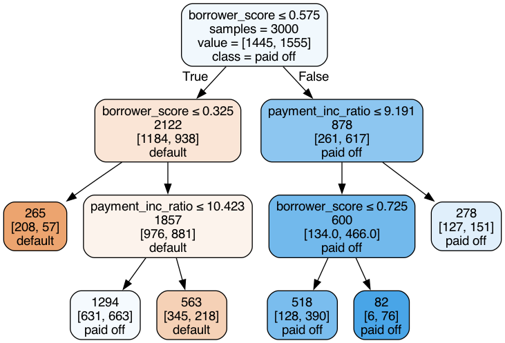

print(textDecisionTree(loan_tree))

node=0 test node: go to node 1 if 0 <= 0.5750000178813934 else to node 6
  node=1 test node: go to node 2 if 0 <= 0.32500000298023224 else to node 3
    node=2 leaf node: [[np.float64(0.785), np.float64(0.215)]]
    node=3 test node: go to node 4 if 1 <= 10.42264986038208 else to node 5
      node=4 leaf node: [[np.float64(0.488), np.float64(0.512)]]
      node=5 leaf node: [[np.float64(0.613), np.float64(0.387)]]
  node=6 test node: go to node 7 if 1 <= 9.19082498550415 else to node 10
    node=7 test node: go to node 8 if 0 <= 0.7249999940395355 else to node 9
      node=8 leaf node: [[np.float64(0.247), np.float64(0.753)]]
      node=9 leaf node: [[np.float64(0.073), np.float64(0.927)]]
    node=10 leaf node: [[np.float64(0.457), np.float64(0.543)]]

Bagging and the Random Forest

Random Forest

predictors = ["borrower_score", "payment_inc_ratio"]
outcome = "outcome"

X = loan3000[predictors]
y = loan3000[outcome]

rf = RandomForestClassifier(n_estimators=500, random_state=1, oob_score=True,
                            n_jobs=4)
rf.fit(X, y)

RandomForestClassifier(n_estimators=500, n_jobs=4, oob_score=True,
                       random_state=1)

In a Jupyter environment, please rerun this cell to show the HTML representation or trust the notebook.
On GitHub, the HTML representation is unable to render, please try loading this page with nbviewer.org.

n_estimator = list(range(20, 505, 5))
oob_scores = []
for n in n_estimator:
    rf = RandomForestClassifier(n_estimators=n, criterion="entropy", n_jobs=4,
                                max_depth=5, random_state=1, oob_score=True)
    rf.fit(X, y)
    oob_scores.append(rf.oob_score_)
df = pd.DataFrame({"n": n_estimator, "oobScore": oob_scores})
df.plot(x="n", y="oobScore")

plt.tight_layout()
plt.show()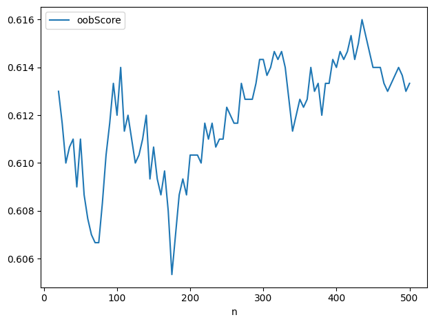

predictions = X.copy()
predictions["prediction"] = rf.predict(X)
predictions.head()

fig, ax = plt.subplots(figsize=(4, 4))

predictions.loc[predictions.prediction == "paid off"].plot(
    x="borrower_score", y="payment_inc_ratio", style=".",
    markerfacecolor="none", markeredgecolor="C1", ax=ax)
predictions.loc[predictions.prediction == "default"].plot(
    x="borrower_score", y="payment_inc_ratio", style="o",
    markerfacecolor="none", markeredgecolor="C0", ax=ax)
ax.legend(["paid off", "default"])
ax.set_xlim(0, 1)
ax.set_ylim(0, 25)
ax.set_xlabel("borrower_score")
ax.set_ylabel("payment_inc_ratio")

plt.tight_layout()
plt.show()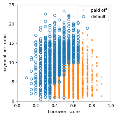

Variable Importance

predictors = ["loan_amnt", "term", "annual_inc", "dti", "payment_inc_ratio",
              "revol_bal", "revol_util", "purpose", "delinq_2yrs_zero",
              "pub_rec_zero", "open_acc", "grade", "emp_length", "purpose_",
              "home_", "emp_len_", "borrower_score"]
outcome = "outcome"

X = pd.get_dummies(loan_data[predictors], drop_first=True)
y = loan_data[outcome]

rf_all = RandomForestClassifier(n_estimators=500, random_state=1, n_jobs=4)
rf_all.fit(X, y)

RandomForestClassifier(n_estimators=500, n_jobs=4, random_state=1)

importances = rf_all.feature_importances_

rng = np.random.default_rng(seed=321)
rf = RandomForestClassifier(n_estimators=500, n_jobs=4)
scores = defaultdict(list)

# cross-validate the scores on a number of different random splits of the data
for _ in range(3):
    train_x, valid_X, train_y, valid_y = train_test_split(X, y, test_size=0.3)
    rf.fit(train_x, train_y)
    acc = metrics.accuracy_score(valid_y, rf.predict(valid_X))
    for column in X.columns:
        X_t = valid_X.copy()
        X_t[column] = rng.permutation(X_t[column].values)
        shuff_acc = metrics.accuracy_score(valid_y, rf.predict(X_t))
        scores[column].append((acc - shuff_acc) / acc)

df = pd.DataFrame({
    "feature": X.columns,
    "Accuracy decrease": [np.mean(scores[column]) for column in X.columns],
    "Gini decrease": rf_all.feature_importances_,
})
df = df.sort_values("Accuracy decrease")

fig, axes = plt.subplots(ncols=2, figsize=(8, 5))
ax = df.plot(kind="barh", x="feature", y="Accuracy decrease",
             legend=False, ax=axes[0])
ax.set_ylabel("")

ax = df.plot(kind="barh", x="feature", y="Gini decrease",
             legend=False, ax=axes[1])
ax.set_ylabel("")
ax.get_yaxis().set_visible(False)

plt.tight_layout()
plt.show()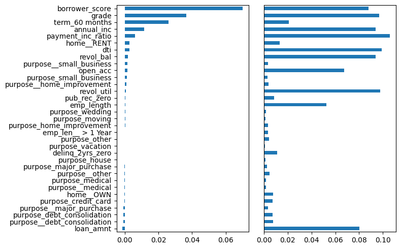

Boosting

XGBoost

predictors = ["borrower_score", "payment_inc_ratio"]
outcome = "outcome"

X = loan3000[predictors]
y = loan3000[outcome]
y = pd.Series([1 if o == "default" else 0 for o in loan3000[outcome]])

xgb = XGBClassifier(objective="binary:logistic", subsample=0.63)
xgb.fit(X, y)

XGBClassifier(base_score=None, booster=None, callbacks=None,
              colsample_bylevel=None, colsample_bynode=None,
              colsample_bytree=None, device=None, early_stopping_rounds=None,
              enable_categorical=False, eval_metric=None, feature_types=None,
              feature_weights=None, gamma=None, grow_policy=None,
              importance_type=None, interaction_constraints=None,
              learning_rate=None, max_bin=None, max_cat_threshold=None,
              max_cat_to_onehot=None, max_delta_step=None, max_depth=None,
              max_leaves=None, min_child_weight=None, missing=nan,
              monotone_constraints=None, multi_strategy=None, n_estimators=None,
              n_jobs=None, num_parallel_tree=None, ...)

xgb_df = X.copy()
xgb_df["prediction"] = ["default" if p == 1 else "paid off"
    for p in xgb.predict(X)]
xgb_df["prob_default"] = xgb.predict_proba(X)[:, 0]

fig, ax = plt.subplots(figsize=(6, 4))

xgb_df.loc[xgb_df.prediction == "paid off"].plot(
    x="borrower_score", y="payment_inc_ratio", style=".",
    markerfacecolor="none", markeredgecolor="C1", ax=ax)
xgb_df.loc[xgb_df.prediction == "default"].plot(
    x="borrower_score", y="payment_inc_ratio", style="o",
    markerfacecolor="none", markeredgecolor="C0", ax=ax)
ax.legend(["paid off", "default"])
ax.set_xlim(0, 1)
ax.set_ylim(0, 25)
ax.set_xlabel("borrower_score")
ax.set_ylabel("payment_inc_ratio")

plt.tight_layout()
plt.show()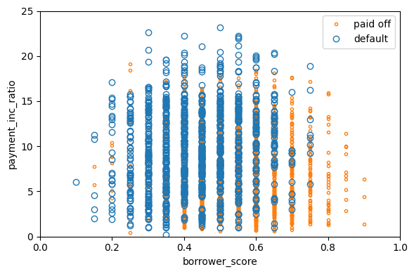

Regularization: Avoiding Overfitting

predictors = ["loan_amnt", "term", "annual_inc", "dti", "payment_inc_ratio",
              "revol_bal", "revol_util", "purpose", "delinq_2yrs_zero",
              "pub_rec_zero", "open_acc", "grade", "emp_length", "purpose_",
              "home_", "emp_len_", "borrower_score"]
outcome = "outcome"

X = pd.get_dummies(loan_data[predictors], drop_first=True)
y = pd.Series([1 if o == "default" else 0 for o in loan_data[outcome]])

train_x, valid_X, train_y, valid_y = train_test_split(X, y, test_size=10000)

xgb_default = XGBClassifier(objective="binary:logistic", n_estimators=250,
                            max_depth=6, reg_lambda=0, learning_rate=0.3,
                            subsample=1)
xgb_default.fit(train_x, train_y)

pred_default = xgb_default.predict_proba(valid_X)[:, 1]
error_default = abs(valid_y - pred_default) > 0.5
print("default: ", np.mean(error_default))

default:  0.364

xgb_penalty = XGBClassifier(objective="binary:logistic", n_estimators=250,
                            max_depth=6, reg_lambda=1000, learning_rate=0.1,
                            subsample=0.63)
xgb_penalty.fit(train_x, train_y)
pred_penalty = xgb_penalty.predict_proba(valid_X)[:, 1]
error_penalty = abs(valid_y - pred_penalty) > 0.5
print("penalty: ", np.mean(error_penalty))

penalty:  0.3274

results = []
for ntree_limit in range(1, 250):
    iteration_range = [1, ntree_limit + 1]
    train_default = xgb_default.predict_proba(train_x,
        iteration_range=iteration_range)[:, 1]
    train_penalty = xgb_penalty.predict_proba(train_x,
        iteration_range=iteration_range)[:, 1]
    pred_default = xgb_default.predict_proba(valid_X,
        iteration_range=iteration_range)[:, 1]
    pred_penalty = xgb_penalty.predict_proba(valid_X,
        iteration_range=iteration_range)[:, 1]
    results.append({
        "iterations": ntree_limit,
        "default train": np.mean(abs(train_y - train_default) > 0.5),
        "penalty train": np.mean(abs(train_y - train_penalty) > 0.5),
        "default test": np.mean(abs(valid_y - pred_default) > 0.5),
        "penalty test": np.mean(abs(valid_y - pred_penalty) > 0.5),
    })

results = pd.DataFrame(results)
results.head()

	iterations	default train	penalty train	default test	penalty test
0	1	0.345962	0.350490	0.3573	0.3531
1	2	0.331306	0.343755	0.3477	0.3479
2	3	0.325081	0.341124	0.3431	0.3415
3	4	0.320836	0.342199	0.3395	0.3404
4	5	0.318686	0.342058	0.3424	0.3396

ax = results.plot(x="iterations", y="default test")
results.plot(x="iterations", y="penalty test", ax=ax)
results.plot(x="iterations", y="default train", ax=ax)
results.plot(x="iterations", y="penalty train", ax=ax)

plt.tight_layout()
plt.show()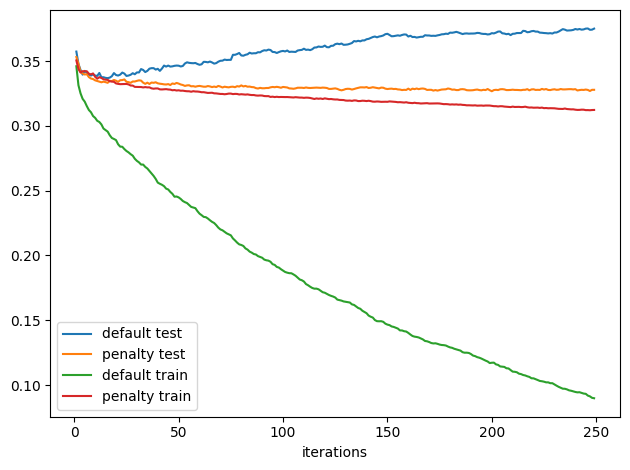

Hyperparameters and Cross-Validation

rng = np.random.default_rng(seed=321)
idx = rng.choice(range(5), size=len(X), replace=True)
error = []
for eta, max_depth in product([0.1, 0.5, 0.9], [3, 6, 9]):
    xgb = XGBClassifier(objective="binary:logistic", n_estimators=250,
                        max_depth=max_depth, learning_rate=eta)
    cv_error = []
    for k in range(5):
        fold_idx = idx == k
        train_x = X.loc[~fold_idx]; train_y = y[~fold_idx]
        valid_X = X.loc[fold_idx]; valid_y = y[fold_idx]

        xgb.fit(train_x, train_y)
        pred = xgb.predict_proba(valid_X)[:, 1]
        cv_error.append(np.mean(abs(valid_y - pred) > 0.5))
    error.append({
        "eta": eta,
        "max_depth": max_depth,
        "avg_error": np.mean(cv_error),
    })
    print(error[-1])
errors = pd.DataFrame(error)

table = errors.pivot_table(index="eta", columns="max_depth", values="avg_error")
print(table * 100)

{'eta': 0.1, 'max_depth': 3, 'avg_error': np.float64(0.32901685739015657)}
{'eta': 0.1, 'max_depth': 6, 'avg_error': np.float64(0.33584569147367743)}
{'eta': 0.1, 'max_depth': 9, 'avg_error': np.float64(0.3465400449213362)}
{'eta': 0.5, 'max_depth': 3, 'avg_error': np.float64(0.3382451177824208)}
{'eta': 0.5, 'max_depth': 6, 'avg_error': np.float64(0.3693638861385647)}
{'eta': 0.5, 'max_depth': 9, 'avg_error': np.float64(0.3704949129861085)}
{'eta': 0.9, 'max_depth': 3, 'avg_error': np.float64(0.34945523328002775)}
{'eta': 0.9, 'max_depth': 6, 'avg_error': np.float64(0.38570299596812696)}
{'eta': 0.9, 'max_depth': 9, 'avg_error': np.float64(0.3824637201456234)}
max_depth          3          6          9
eta                                       
0.1        32.901686  33.584569  34.654004
0.5        33.824512  36.936389  37.049491
0.9        34.945523  38.570300  38.246372

Supplementary Material

Figure 6-2. KNN prediction of loan default using two variables: debt-to-income ratio and loan-payment-to-income ratio

predictors = ["payment_inc_ratio", "dti"]
outcome = "outcome"
newloan = loan200.loc[0:0, predictors]
X = loan200.loc[1:, predictors]
y = loan200.loc[1:, outcome]

knn = KNeighborsClassifier(n_neighbors=20)
knn.fit(X, y)

nbrs = knn.kneighbors(newloan)
maxDistance = np.max(nbrs[0][0])

fig, ax = plt.subplots(figsize=(4, 4))
sns.scatterplot(x="payment_inc_ratio", y="dti", style="outcome",
                hue="outcome", data=loan200, alpha=0.3, ax=ax)
sns.scatterplot(x="payment_inc_ratio", y="dti", style="outcome",
                hue="outcome",
                data=pd.concat([loan200.loc[0:0, :], loan200.loc[nbrs[1][0] + 1, :]]),
                ax=ax, legend=False)
ellipse = Ellipse(xy=newloan.to_numpy()[0],
                  width=2 * maxDistance, height=2 * maxDistance,
                  edgecolor="black", fc="None", lw=1)
ax.add_patch(ellipse)
ax.set_xlim(3, 16)
ax.set_ylim(15, 30)

plt.tight_layout()
plt.show()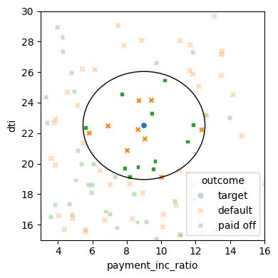

Figure 6-4. The first five rules for a simple tree model fit to the loan data

fig, ax = plt.subplots(figsize=(6, 4))

loan3000.loc[loan3000.outcome == "paid off"].plot(
    x="borrower_score", y="payment_inc_ratio", style=".",
    markerfacecolor="none", markeredgecolor="C1", ax=ax)
loan3000.loc[loan3000.outcome == "default"].plot(
    x="borrower_score", y="payment_inc_ratio", style="o",
    markerfacecolor="none", markeredgecolor="C0", ax=ax)
ax.legend(["paid off", "default"])
ax.set_xlim(0, 1)
ax.set_ylim(0, 25)
ax.set_xlabel("borrower_score")
ax.set_ylabel("payment_inc_ratio")

x0 = 0.575
x1a = 0.325; y1b = 9.191
y2a = 10.423; x2b = 0.725
ax.plot((x0, x0), (0, 25), color="grey")
ax.plot((x1a, x1a), (0, 25), color="grey")
ax.plot((x0, 1), (y1b, y1b), color="grey")
ax.plot((x1a, x0), (y2a, y2a), color="grey")
ax.plot((x2b, x2b), (0, y1b), color="grey")

labels = [("default", (x1a / 2, 25 / 2)),
          ("default", ((x0 + x1a) / 2, (25 + y2a) / 2)),
          ("paid off", ((x0 + x1a) / 2, y2a / 2)),
          ("paid off", ((1 + x0) / 2, (y1b + 25) / 2)),
          ("paid off", ((1 + x2b) / 2, (y1b + 0) / 2)),
          ("paid off", ((x0 + x2b) / 2, (y1b + 0) / 2)),
         ]
for label, (x, y) in labels:
    ax.text(x, y, label, bbox={"facecolor": "white"},
            verticalalignment="center", horizontalalignment="center")

plt.tight_layout()
plt.show()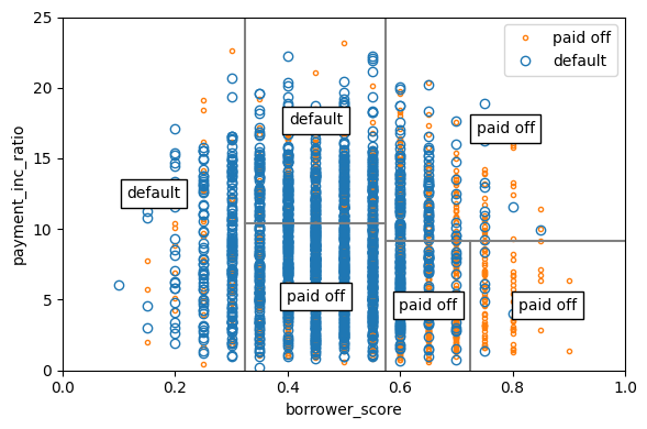

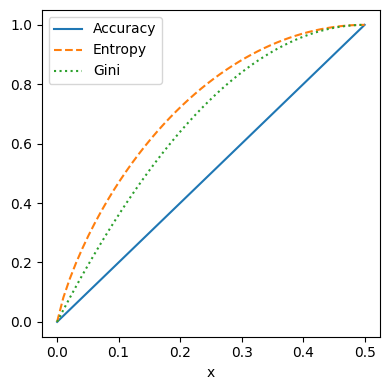
Figure 6-5. Gini impurity and entropy measures

def entropy_function(x):
    if x == 0:
        return 0
    return -x * math.log2(x) - (1 - x) * math.log2(1 - x)

def gini_function(x):
    return x * (1 - x)

x = np.linspace(0, 0.5, 50)
impure = pd.DataFrame({
    "x": x,
    "Accuracy": 2 * x,
    "Gini": [gini_function(xi) / gini_function(0.5) for xi in x],
    "Entropy": [entropy_function(xi) for xi in x],
})

fig, ax = plt.subplots(figsize=(4, 4))

impure.plot(x="x", y="Accuracy", ax=ax, linestyle="solid")
impure.plot(x="x", y="Entropy", ax=ax, linestyle="--")
impure.plot(x="x", y="Gini", ax=ax, linestyle=":")

plt.tight_layout()
plt.show()

	n_estimators n_estimators: int, default=100 The number of trees in the forest. .. versionchanged:: 0.22 The default value of ``n_estimators`` changed from 10 to 100 in 0.22.	500
	criterion criterion: {"gini", "entropy", "log_loss"}, default="gini" The function to measure the quality of a split. Supported criteria are "gini" for the Gini impurity and "log_loss" and "entropy" both for the Shannon information gain, see :ref:`tree_mathematical_formulation`. Note: This parameter is tree-specific.	'gini'
	max_depth max_depth: int, default=None The maximum depth of the tree. If None, then nodes are expanded until all leaves are pure or until all leaves contain less than min_samples_split samples.	None
	min_samples_split min_samples_split: int or float, default=2 The minimum number of samples required to split an internal node: - If int, then consider `min_samples_split` as the minimum number. - If float, then `min_samples_split` is a fraction and `ceil(min_samples_split * n_samples)` are the minimum number of samples for each split. .. versionchanged:: 0.18 Added float values for fractions.	2
	min_samples_leaf min_samples_leaf: int or float, default=1 The minimum number of samples required to be at a leaf node. A split point at any depth will only be considered if it leaves at least ``min_samples_leaf`` training samples in each of the left and right branches. This may have the effect of smoothing the model, especially in regression. - If int, then consider `min_samples_leaf` as the minimum number. - If float, then `min_samples_leaf` is a fraction and `ceil(min_samples_leaf * n_samples)` are the minimum number of samples for each node. .. versionchanged:: 0.18 Added float values for fractions.	1
	min_weight_fraction_leaf min_weight_fraction_leaf: float, default=0.0 The minimum weighted fraction of the sum total of weights (of all the input samples) required to be at a leaf node. Samples have equal weight when sample_weight is not provided.	0.0
	max_features max_features: {"sqrt", "log2", None}, int or float, default="sqrt" The number of features to consider when looking for the best split: - If int, then consider `max_features` features at each split. - If float, then `max_features` is a fraction and `max(1, int(max_features * n_features_in_))` features are considered at each split. - If "sqrt", then `max_features=sqrt(n_features)`. - If "log2", then `max_features=log2(n_features)`. - If None, then `max_features=n_features`. .. versionchanged:: 1.1 The default of `max_features` changed from `"auto"` to `"sqrt"`. Note: the search for a split does not stop until at least one valid partition of the node samples is found, even if it requires to effectively inspect more than ``max_features`` features.	'sqrt'
	max_leaf_nodes max_leaf_nodes: int, default=None Grow trees with ``max_leaf_nodes`` in best-first fashion. Best nodes are defined as relative reduction in impurity. If None then unlimited number of leaf nodes.	None
	min_impurity_decrease min_impurity_decrease: float, default=0.0 A node will be split if this split induces a decrease of the impurity greater than or equal to this value. The weighted impurity decrease equation is the following:: N_t / N * (impurity - N_t_R / N_t * right_impurity - N_t_L / N_t * left_impurity) where ``N`` is the total number of samples, ``N_t`` is the number of samples at the current node, ``N_t_L`` is the number of samples in the left child, and ``N_t_R`` is the number of samples in the right child. ``N``, ``N_t``, ``N_t_R`` and ``N_t_L`` all refer to the weighted sum, if ``sample_weight`` is passed. .. versionadded:: 0.19	0.0
	bootstrap bootstrap: bool, default=True Whether bootstrap samples are used when building trees. If False, the whole dataset is used to build each tree.	True
	oob_score oob_score: bool or callable, default=False Whether to use out-of-bag samples to estimate the generalization score. By default, :func:`~sklearn.metrics.accuracy_score` is used. Provide a callable with signature `metric(y_true, y_pred)` to use a custom metric. Only available if `bootstrap=True`. For an illustration of out-of-bag (OOB) error estimation, see the example :ref:`sphx_glr_auto_examples_ensemble_plot_ensemble_oob.py`.	True
	n_jobs n_jobs: int, default=None The number of jobs to run in parallel. :meth:`fit`, :meth:`predict`, :meth:`decision_path` and :meth:`apply` are all parallelized over the trees. ``None`` means 1 unless in a :obj:`joblib.parallel_backend` context. ``-1`` means using all processors. See :term:`Glossary ` for more details.	4
	random_state random_state: int, RandomState instance or None, default=None Controls both the randomness of the bootstrapping of the samples used when building trees (if ``bootstrap=True``) and the sampling of the features to consider when looking for the best split at each node (if ``max_features < n_features``). See :term:`Glossary ` for details.	1
	verbose verbose: int, default=0 Controls the verbosity when fitting and predicting.	0
	warm_start warm_start: bool, default=False When set to ``True``, reuse the solution of the previous call to fit and add more estimators to the ensemble, otherwise, just fit a whole new forest. See :term:`Glossary ` and :ref:`tree_ensemble_warm_start` for details.	False
	class_weight class_weight: {"balanced", "balanced_subsample"}, dict or list of dicts, default=None Weights associated with classes in the form ``{class_label: weight}``. If not given, all classes are supposed to have weight one. For multi-output problems, a list of dicts can be provided in the same order as the columns of y. Note that for multioutput (including multilabel) weights should be defined for each class of every column in its own dict. For example, for four-class multilabel classification weights should be [{0: 1, 1: 1}, {0: 1, 1: 5}, {0: 1, 1: 1}, {0: 1, 1: 1}] instead of [{1:1}, {2:5}, {3:1}, {4:1}]. The "balanced" mode uses the values of y to automatically adjust weights inversely proportional to class frequencies in the input data as ``n_samples / (n_classes * np.bincount(y))`` The "balanced_subsample" mode is the same as "balanced" except that weights are computed based on the bootstrap sample for every tree grown. For multi-output, the weights of each column of y will be multiplied. Note that these weights will be multiplied with sample_weight (passed through the fit method) if sample_weight is specified.	None
	ccp_alpha ccp_alpha: non-negative float, default=0.0 Complexity parameter used for Minimal Cost-Complexity Pruning. The subtree with the largest cost complexity that is smaller than ``ccp_alpha`` will be chosen. By default, no pruning is performed. See :ref:`minimal_cost_complexity_pruning` for details. See :ref:`sphx_glr_auto_examples_tree_plot_cost_complexity_pruning.py` for an example of such pruning. .. versionadded:: 0.22	0.0
	max_samples max_samples: int or float, default=None If bootstrap is True, the number of samples to draw from X to train each base estimator. - If None (default), then draw `X.shape[0]` samples. - If int, then draw `max_samples` samples. - If float, then draw `max(round(n_samples * max_samples), 1)` samples. Thus, `max_samples` should be in the interval `(0.0, 1.0]`. .. versionadded:: 0.22	None
	monotonic_cst monotonic_cst: array-like of int of shape (n_features), default=None Indicates the monotonicity constraint to enforce on each feature. - 1: monotonic increase - 0: no constraint - -1: monotonic decrease If monotonic_cst is None, no constraints are applied. Monotonicity constraints are not supported for: - multiclass classifications (i.e. when `n_classes > 2`), - multioutput classifications (i.e. when `n_outputs_ > 1`), - classifications trained on data with missing values. The constraints hold over the probability of the positive class. Read more in the :ref:`User Guide `. .. versionadded:: 1.4	None

	n_estimators n_estimators: int, default=100 The number of trees in the forest. .. versionchanged:: 0.22 The default value of ``n_estimators`` changed from 10 to 100 in 0.22.	500
	criterion criterion: {"gini", "entropy", "log_loss"}, default="gini" The function to measure the quality of a split. Supported criteria are "gini" for the Gini impurity and "log_loss" and "entropy" both for the Shannon information gain, see :ref:`tree_mathematical_formulation`. Note: This parameter is tree-specific.	'gini'
	max_depth max_depth: int, default=None The maximum depth of the tree. If None, then nodes are expanded until all leaves are pure or until all leaves contain less than min_samples_split samples.	None
	min_samples_split min_samples_split: int or float, default=2 The minimum number of samples required to split an internal node: - If int, then consider `min_samples_split` as the minimum number. - If float, then `min_samples_split` is a fraction and `ceil(min_samples_split * n_samples)` are the minimum number of samples for each split. .. versionchanged:: 0.18 Added float values for fractions.	2
	min_samples_leaf min_samples_leaf: int or float, default=1 The minimum number of samples required to be at a leaf node. A split point at any depth will only be considered if it leaves at least ``min_samples_leaf`` training samples in each of the left and right branches. This may have the effect of smoothing the model, especially in regression. - If int, then consider `min_samples_leaf` as the minimum number. - If float, then `min_samples_leaf` is a fraction and `ceil(min_samples_leaf * n_samples)` are the minimum number of samples for each node. .. versionchanged:: 0.18 Added float values for fractions.	1
	min_weight_fraction_leaf min_weight_fraction_leaf: float, default=0.0 The minimum weighted fraction of the sum total of weights (of all the input samples) required to be at a leaf node. Samples have equal weight when sample_weight is not provided.	0.0
	max_features max_features: {"sqrt", "log2", None}, int or float, default="sqrt" The number of features to consider when looking for the best split: - If int, then consider `max_features` features at each split. - If float, then `max_features` is a fraction and `max(1, int(max_features * n_features_in_))` features are considered at each split. - If "sqrt", then `max_features=sqrt(n_features)`. - If "log2", then `max_features=log2(n_features)`. - If None, then `max_features=n_features`. .. versionchanged:: 1.1 The default of `max_features` changed from `"auto"` to `"sqrt"`. Note: the search for a split does not stop until at least one valid partition of the node samples is found, even if it requires to effectively inspect more than ``max_features`` features.	'sqrt'
	max_leaf_nodes max_leaf_nodes: int, default=None Grow trees with ``max_leaf_nodes`` in best-first fashion. Best nodes are defined as relative reduction in impurity. If None then unlimited number of leaf nodes.	None
	min_impurity_decrease min_impurity_decrease: float, default=0.0 A node will be split if this split induces a decrease of the impurity greater than or equal to this value. The weighted impurity decrease equation is the following:: N_t / N * (impurity - N_t_R / N_t * right_impurity - N_t_L / N_t * left_impurity) where ``N`` is the total number of samples, ``N_t`` is the number of samples at the current node, ``N_t_L`` is the number of samples in the left child, and ``N_t_R`` is the number of samples in the right child. ``N``, ``N_t``, ``N_t_R`` and ``N_t_L`` all refer to the weighted sum, if ``sample_weight`` is passed. .. versionadded:: 0.19	0.0
	bootstrap bootstrap: bool, default=True Whether bootstrap samples are used when building trees. If False, the whole dataset is used to build each tree.	True
	oob_score oob_score: bool or callable, default=False Whether to use out-of-bag samples to estimate the generalization score. By default, :func:`~sklearn.metrics.accuracy_score` is used. Provide a callable with signature `metric(y_true, y_pred)` to use a custom metric. Only available if `bootstrap=True`. For an illustration of out-of-bag (OOB) error estimation, see the example :ref:`sphx_glr_auto_examples_ensemble_plot_ensemble_oob.py`.	False
	n_jobs n_jobs: int, default=None The number of jobs to run in parallel. :meth:`fit`, :meth:`predict`, :meth:`decision_path` and :meth:`apply` are all parallelized over the trees. ``None`` means 1 unless in a :obj:`joblib.parallel_backend` context. ``-1`` means using all processors. See :term:`Glossary ` for more details.	4
	random_state random_state: int, RandomState instance or None, default=None Controls both the randomness of the bootstrapping of the samples used when building trees (if ``bootstrap=True``) and the sampling of the features to consider when looking for the best split at each node (if ``max_features < n_features``). See :term:`Glossary ` for details.	1
	verbose verbose: int, default=0 Controls the verbosity when fitting and predicting.	0
	warm_start warm_start: bool, default=False When set to ``True``, reuse the solution of the previous call to fit and add more estimators to the ensemble, otherwise, just fit a whole new forest. See :term:`Glossary ` and :ref:`tree_ensemble_warm_start` for details.	False
	class_weight class_weight: {"balanced", "balanced_subsample"}, dict or list of dicts, default=None Weights associated with classes in the form ``{class_label: weight}``. If not given, all classes are supposed to have weight one. For multi-output problems, a list of dicts can be provided in the same order as the columns of y. Note that for multioutput (including multilabel) weights should be defined for each class of every column in its own dict. For example, for four-class multilabel classification weights should be [{0: 1, 1: 1}, {0: 1, 1: 5}, {0: 1, 1: 1}, {0: 1, 1: 1}] instead of [{1:1}, {2:5}, {3:1}, {4:1}]. The "balanced" mode uses the values of y to automatically adjust weights inversely proportional to class frequencies in the input data as ``n_samples / (n_classes * np.bincount(y))`` The "balanced_subsample" mode is the same as "balanced" except that weights are computed based on the bootstrap sample for every tree grown. For multi-output, the weights of each column of y will be multiplied. Note that these weights will be multiplied with sample_weight (passed through the fit method) if sample_weight is specified.	None
	ccp_alpha ccp_alpha: non-negative float, default=0.0 Complexity parameter used for Minimal Cost-Complexity Pruning. The subtree with the largest cost complexity that is smaller than ``ccp_alpha`` will be chosen. By default, no pruning is performed. See :ref:`minimal_cost_complexity_pruning` for details. See :ref:`sphx_glr_auto_examples_tree_plot_cost_complexity_pruning.py` for an example of such pruning. .. versionadded:: 0.22	0.0
	max_samples max_samples: int or float, default=None If bootstrap is True, the number of samples to draw from X to train each base estimator. - If None (default), then draw `X.shape[0]` samples. - If int, then draw `max_samples` samples. - If float, then draw `max(round(n_samples * max_samples), 1)` samples. Thus, `max_samples` should be in the interval `(0.0, 1.0]`. .. versionadded:: 0.22	None
	monotonic_cst monotonic_cst: array-like of int of shape (n_features), default=None Indicates the monotonicity constraint to enforce on each feature. - 1: monotonic increase - 0: no constraint - -1: monotonic decrease If monotonic_cst is None, no constraints are applied. Monotonicity constraints are not supported for: - multiclass classifications (i.e. when `n_classes > 2`), - multioutput classifications (i.e. when `n_outputs_ > 1`), - classifications trained on data with missing values. The constraints hold over the probability of the positive class. Read more in the :ref:`User Guide `. .. versionadded:: 1.4	None