Chapter 4: Regression and Prediction

2019-2026 Peter C. Bruce, Andrew Bruce, Peter Gedeck

from mlxtend.feature_selection import SequentialFeatureSelector
from pygam import LinearGAM, s, l
from scipy.stats import linregress
from sklearn.linear_model import Lasso, LassoLars, LassoCV, LassoLarsCV
from sklearn.linear_model import LinearRegression
from sklearn.metrics import mean_squared_error, r2_score
from sklearn.pipeline import Pipeline
from sklearn.preprocessing import StandardScaler
from statsmodels.gam.api import GLMGam, BSplines
from statsmodels.stats.outliers_influence import OLSInfluence
import matplotlib.pyplot as plt
import numpy as np
import pandas as pd
import random
import seaborn as sns
import statsmodels.api as sm
import statsmodels.formula.api as smf

random.seed(123)

# Location of the data files. Adjust this path if you keep the data
# files in a different directory.
from pathlib import Path
DATA_DIR = Path('../data')

Regression and Prediction

Simple Linear Regression

The Regression Equation

lung = pd.read_csv(DATA_DIR / "LungDisease.csv")

predictors = ["Exposure"]
outcome = "PEFR"

model = LinearRegression()
model.fit(lung[predictors], lung[outcome])

print(f"Intercept: {model.intercept_:.3f}")
print(f"Coefficient Exposure: {model.coef_[0]:.3f}")

Intercept: 424.583
Coefficient Exposure: -4.185

Fitted Values and Residuals

fitted = model.predict(lung[predictors])
residuals = lung[outcome] - fitted

Multiple Linear Regression

Example: King County Housing Data

house = pd.read_csv(DATA_DIR / "house_sales.csv")

subset = ["AdjSalePrice", "SqFtTotLiving", "SqFtLot", "Bathrooms",
          "Bedrooms", "BldgGrade"]
house[subset].head()

	AdjSalePrice	SqFtTotLiving	SqFtLot	Bathrooms	Bedrooms	BldgGrade
0	300805.0	2400	9373	3.00	6	7
1	1076162.0	3764	20156	3.75	4	10
2	761805.0	2060	26036	1.75	4	8
3	442065.0	3200	8618	3.75	5	7
4	297065.0	1720	8620	1.75	4	7

predictors = ["SqFtTotLiving", "SqFtLot", "Bathrooms", "Bedrooms", "BldgGrade"]
outcome = "AdjSalePrice"

house_lm = LinearRegression()
house_lm.fit(house[predictors], house[outcome])

LinearRegression()

In a Jupyter environment, please rerun this cell to show the HTML representation or trust the notebook.
On GitHub, the HTML representation is unable to render, please try loading this page with nbviewer.org.

print(f"Intercept: {house_lm.intercept_:.3f}")
print("Coefficients:")
for name, coef in zip(house_lm.feature_names_in_, house_lm.coef_, strict=True):
    print(f" {name}: {coef}")

Intercept: -521871.368
Coefficients:
 SqFtTotLiving: 228.83060360240785
 SqFtLot: -0.060466820653060145
 Bathrooms: -19442.840398321074
 Bedrooms: -47769.9551852142
 BldgGrade: 106106.96307898112

Assessing the Model

fitted = house_lm.predict(house[predictors])
RMSE = np.sqrt(mean_squared_error(house[outcome], fitted))
r2 = r2_score(house[outcome], fitted)
print(f"RMSE: {RMSE:.0f}")
print(f"r2: {r2:.4f}")

RMSE: 261220
r2: 0.5406

model = sm.OLS(house[outcome], sm.add_constant(house[predictors]))
results = model.fit()
results.summary()

OLS Regression Results
Dep. Variable:	AdjSalePrice	R-squared:	0.541
Model:	OLS	Adj. R-squared:	0.540
Method:	Least Squares	F-statistic:	5338.
Date:	Tue, 09 Jun 2026	Prob (F-statistic):	0.00
Time:	18:18:15	Log-Likelihood:	-3.1517e+05
No. Observations:	22687	AIC:	6.304e+05
Df Residuals:	22681	BIC:	6.304e+05
Df Model:	5
Covariance Type:	nonrobust

	coef	std err	t	P>\|t\|	[0.025	0.975]
const	-5.219e+05	1.57e+04	-33.342	0.000	-5.53e+05	-4.91e+05
SqFtTotLiving	228.8306	3.899	58.694	0.000	221.189	236.472
SqFtLot	-0.0605	0.061	-0.988	0.323	-0.180	0.059
Bathrooms	-1.944e+04	3625.388	-5.363	0.000	-2.65e+04	-1.23e+04
Bedrooms	-4.777e+04	2489.732	-19.187	0.000	-5.27e+04	-4.29e+04
BldgGrade	1.061e+05	2396.445	44.277	0.000	1.01e+05	1.11e+05

Omnibus:	29676.557	Durbin-Watson:	1.247
Prob(Omnibus):	0.000	Jarque-Bera (JB):	19390738.346
Skew:	6.889	Prob(JB):	0.00
Kurtosis:	145.559	Cond. No.	2.86e+05

Notes:
[1] Standard Errors assume that the covariance matrix of the errors is correctly specified.
[2] The condition number is large, 2.86e+05. This might indicate that there are
strong multicollinearity or other numerical problems.

Model Selection and Stepwise Regression

predictors = ["SqFtTotLiving", "SqFtLot", "Bathrooms", "Bedrooms", "BldgGrade",
              "PropertyType", "NbrLivingUnits", "SqFtFinBasement", "YrBuilt",
              "YrRenovated", "NewConstruction"]

X = pd.get_dummies(house[predictors], drop_first=True, dtype=int)
X["NewConstruction"] = [1 if nc else 0 for nc in X["NewConstruction"]]

house_full = sm.OLS(house[outcome], sm.add_constant(X))
results = house_full.fit()
results.summary()

OLS Regression Results
Dep. Variable:	AdjSalePrice	R-squared:	0.595
Model:	OLS	Adj. R-squared:	0.594
Method:	Least Squares	F-statistic:	2771.
Date:	Tue, 09 Jun 2026	Prob (F-statistic):	0.00
Time:	18:18:15	Log-Likelihood:	-3.1375e+05
No. Observations:	22687	AIC:	6.275e+05
Df Residuals:	22674	BIC:	6.276e+05
Df Model:	12
Covariance Type:	nonrobust

	coef	std err	t	P>\|t\|	[0.025	0.975]
const	6.182e+06	1.55e+05	39.902	0.000	5.88e+06	6.49e+06
SqFtTotLiving	198.6364	4.234	46.920	0.000	190.338	206.934
SqFtLot	0.0771	0.058	1.330	0.184	-0.037	0.191
Bathrooms	4.286e+04	3808.114	11.255	0.000	3.54e+04	5.03e+04
Bedrooms	-5.187e+04	2396.904	-21.638	0.000	-5.66e+04	-4.72e+04
BldgGrade	1.373e+05	2441.242	56.228	0.000	1.32e+05	1.42e+05
NbrLivingUnits	5723.8438	1.76e+04	0.326	0.744	-2.87e+04	4.01e+04
SqFtFinBasement	7.0611	4.627	1.526	0.127	-2.009	16.131
YrBuilt	-3574.2210	77.228	-46.282	0.000	-3725.593	-3422.849
YrRenovated	-2.5311	3.924	-0.645	0.519	-10.222	5.160
NewConstruction	-2489.1122	5936.692	-0.419	0.675	-1.41e+04	9147.211
PropertyType_Single Family	2.997e+04	2.61e+04	1.149	0.251	-2.12e+04	8.11e+04
PropertyType_Townhouse	9.286e+04	2.7e+04	3.438	0.001	3.99e+04	1.46e+05

Omnibus:	31006.128	Durbin-Watson:	1.393
Prob(Omnibus):	0.000	Jarque-Bera (JB):	26251977.078
Skew:	7.427	Prob(JB):	0.00
Kurtosis:	168.984	Cond. No.	2.98e+06

Notes:
[1] Standard Errors assume that the covariance matrix of the errors is correctly specified.
[2] The condition number is large, 2.98e+06. This might indicate that there are
strong multicollinearity or other numerical problems.

sfs_stepwise = SequentialFeatureSelector(LinearRegression(),
    k_features=(1, 11),
    forward=True, floating=True,
    cv=5, scoring="neg_root_mean_squared_error", n_jobs=-1)

sfs_stepwise.fit(X, house[outcome])
print(sfs_stepwise.k_feature_names_)

('SqFtTotLiving', 'Bathrooms', 'Bedrooms', 'BldgGrade', 'YrBuilt', 'PropertyType_Single Family', 'PropertyType_Townhouse')

step_lm = Pipeline([
    ("sfs", SequentialFeatureSelector(LinearRegression(),
        k_features=(1, 12), forward=False, floating=True,
        cv=5, scoring="neg_root_mean_squared_error", n_jobs=-1)),
    ("model", LinearRegression()),
])
step_lm.fit(X, house[outcome])

/Users/petergedeck/cdd/practical-statistics-for-data-scientists-code-3e/.venv/lib/python3.13/site-packages/sklearn/externals/_numpydoc/docscrape.py:203: UserWarning: potentially wrong underline length... 
Examples 
----------- in 
Sequential Feature Selection for Classification and Regression.
...
  while not self._is_at_section() and not self._doc.eof():

Pipeline(steps=[('sfs',
                 SequentialFeatureSelector(estimator=LinearRegression(),
                                           floating=True, forward=False,
                                           k_features=(1, 12), n_jobs=-1,
                                           scoring='neg_root_mean_squared_error')),
                ('model', LinearRegression())])

Weighted Regression

house["Year"] = [int(date.split("-")[0]) for date in house.DocumentDate]
house["Weight"] = house.Year - 2005

predictors = ["SqFtTotLiving", "SqFtLot", "Bathrooms", "Bedrooms", "BldgGrade"]
outcome = "AdjSalePrice"

house_wt = LinearRegression()
house_wt.fit(house[predictors], house[outcome], sample_weight=house.Weight)

LinearRegression()

pd.concat([
    pd.DataFrame({
        "predictor": predictors,
        "house_lm": house_lm.coef_,
        "house_wt": house_wt.coef_,
    }),
    pd.DataFrame({
        "predictor": ["intercept"],
        "house_lm": house_lm.intercept_,
        "house_wt": house_wt.intercept_,
    }),
])

	predictor	house_lm	house_wt
0	SqFtTotLiving	228.830604	245.024089
1	SqFtLot	-0.060467	-0.292415
2	Bathrooms	-19442.840398	-26085.970109
3	Bedrooms	-47769.955185	-53608.876436
4	BldgGrade	106106.963079	115242.434726
0	intercept	-521871.368188	-584189.329446

Factor Variables in Regression

Dummy Variables Representation

house.PropertyType.head()

0        Multiplex
1    Single Family
2    Single Family
3    Single Family
4    Single Family
Name: PropertyType, dtype: str

print(pd.get_dummies(house["PropertyType"]).head())
print(pd.get_dummies(house["PropertyType"], drop_first=True).head())

   Multiplex  Single Family  Townhouse
0       True          False      False
1      False           True      False
2      False           True      False
3      False           True      False
4      False           True      False
   Single Family  Townhouse
0          False      False
1           True      False
2           True      False
3           True      False
4           True      False

predictors = ["SqFtTotLiving", "SqFtLot", "Bathrooms", "Bedrooms",
              "BldgGrade", "PropertyType"]

X = pd.get_dummies(house[predictors], drop_first=True, dtype=int)

house_lm_factor = LinearRegression()
house_lm_factor.fit(X, house[outcome])

print(f"Intercept: {house_lm_factor.intercept_:.3f}")
print("Coefficients:")
for name, coef in zip(X.columns, house_lm_factor.coef_, strict=True):
    print(f" {name}: {coef}")

Intercept: -446841.366
Coefficients:
 SqFtTotLiving: 223.37362892503833
 SqFtLot: -0.07036798136811658
 Bathrooms: -15979.013473415354
 Bedrooms: -50889.73218483002
 BldgGrade: 109416.30516146205
 PropertyType_Single Family: -84678.21629549282
 PropertyType_Townhouse: -115121.97921609184

Factor Variables with Many Levels

pd.DataFrame(house["ZipCode"].value_counts()).transpose()

ZipCode	98038	98103	98042	98115	98117	98052	98034	98033	98059	98074	...	98051	98024	98354	98050	98057	98288	98224	98068	98113	98043
count	788	671	641	620	619	614	575	517	513	502	...	32	31	9	7	4	4	3	1	1	1

1 rows × 80 columns

house = pd.read_csv(DATA_DIR / "house_sales.csv")
predictors = ["SqFtTotLiving", "SqFtLot", "Bathrooms", "Bedrooms", "BldgGrade"]
outcome = "AdjSalePrice"
house_lm = LinearRegression()
house_lm.fit(house[predictors], house[outcome])

zip_groups = pd.DataFrame([
    *pd.DataFrame({
        "ZipCode": house["ZipCode"],
        "residual": house[outcome] - house_lm.predict(house[predictors]),
    })
    .groupby(["ZipCode"])[["ZipCode", "residual"]]
    .apply(lambda x: {
        "ZipCode": x.iloc[0, 0],
        "count": len(x),
        "median_residual": x.residual.median(),
    }),
]).sort_values("median_residual")
zip_groups["cum_count"] = np.cumsum(zip_groups["count"])
zip_groups["ZipGroup"] = pd.qcut(zip_groups["cum_count"], 5, labels=False,
                                 retbins=False)

to_join = zip_groups[["ZipCode", "ZipGroup"]].set_index("ZipCode")
house = house.join(to_join, on="ZipCode")
house["ZipGroup"] = house["ZipGroup"].astype("category")

print(zip_groups.head())
print(zip_groups.ZipGroup.value_counts().sort_index())

    ZipCode  count  median_residual  cum_count  ZipGroup
36    98057      4   -537321.644462          4         0
27    98043      1   -307661.343614          5         0
46    98092    289   -193569.183599        294         0
23    98038    788   -150066.477035       1082         0
31    98051     32   -142352.869593       1114         0
ZipGroup
0    16
1    16
2    16
3    16
4    16
Name: count, dtype: int64

Interpreting the Regression Equation

Correlated Predictors

print(f"Intercept: {step_lm.named_steps['model'].intercept_:.3f}")
print("Coefficients:")
for name, coef in zip(step_lm.named_steps["sfs"].k_feature_names_,
                      step_lm.named_steps["model"].coef_, strict=True):
    print(f"  {name}: {coef}")

Intercept: 6259055.855
Coefficients:
  SqFtTotLiving: 201.65789971342235
  Bathrooms: 42787.933811708994
  Bedrooms: -51742.8382076272
  BldgGrade: 136309.59662237618
  YrBuilt: -3605.8233277869685
  PropertyType_Single Family: 24105.25018215709
  PropertyType_Townhouse: 87589.26527129347

predictors = ["Bedrooms", "BldgGrade", "PropertyType", "YrBuilt"]
outcome = "AdjSalePrice"

X = pd.get_dummies(house[predictors], drop_first=True, dtype=int)

reduced_lm = LinearRegression()
reduced_lm.fit(X, house[outcome])

LinearRegression()

print(f"Intercept: {reduced_lm.intercept_:.3f}")
print("Coefficients:")
for name, coef in zip(X.columns, reduced_lm.coef_, strict=True):
    print(f" {name}: {coef}")

Intercept: 4913973.344
Coefficients:
 Bedrooms: 27150.53723021958
 BldgGrade: 248997.7936621269
 YrBuilt: -3211.7448621551166
 PropertyType_Single Family: -19898.49534050195
 PropertyType_Townhouse: -47355.43687334422

Confounding Variables

predictors = ["SqFtTotLiving", "SqFtLot", "Bathrooms", "Bedrooms",
              "BldgGrade", "PropertyType", "ZipGroup"]
outcome = "AdjSalePrice"

X = pd.get_dummies(house[predictors], drop_first=True, dtype=int)

confounding_lm = LinearRegression()
confounding_lm.fit(X, house[outcome])

print(f"Intercept: {confounding_lm.intercept_:.3f}")
print("Coefficients:")
for name, coef in zip(X.columns, confounding_lm.coef_, strict=True):
    print(f" {name}: {coef}")

Intercept: -666637.469
Coefficients:
 SqFtTotLiving: 210.61266005580163
 SqFtLot: 0.4549871385466008
 Bathrooms: 5928.425640001413
 Bedrooms: -41682.871840744534
 BldgGrade: 98541.18352725999
 PropertyType_Single Family: 19323.625287919574
 PropertyType_Townhouse: -78198.72092762378
 ZipGroup_1: 53317.17330659807
 ZipGroup_2: 116251.5888356354
 ZipGroup_3: 178360.53178793358
 ZipGroup_4: 338408.6018565202

Interactions and Main Effects

model = smf.ols(formula="AdjSalePrice ~ SqFtTotLiving*ZipGroup + SqFtLot + "
     "Bathrooms + Bedrooms + BldgGrade + PropertyType", data=house)
results = model.fit()
results.summary()

OLS Regression Results
Dep. Variable:	AdjSalePrice	R-squared:	0.682
Model:	OLS	Adj. R-squared:	0.682
Method:	Least Squares	F-statistic:	3247.
Date:	Tue, 09 Jun 2026	Prob (F-statistic):	0.00
Time:	18:18:23	Log-Likelihood:	-3.1098e+05
No. Observations:	22687	AIC:	6.220e+05
Df Residuals:	22671	BIC:	6.221e+05
Df Model:	15
Covariance Type:	nonrobust

	coef	std err	t	P>\|t\|	[0.025	0.975]
Intercept	-4.853e+05	2.05e+04	-23.701	0.000	-5.25e+05	-4.45e+05
ZipGroup[T.1]	-1.113e+04	1.34e+04	-0.830	0.407	-3.74e+04	1.52e+04
ZipGroup[T.2]	2.032e+04	1.18e+04	1.717	0.086	-2877.441	4.35e+04
ZipGroup[T.3]	2.05e+04	1.21e+04	1.697	0.090	-3180.870	4.42e+04
ZipGroup[T.4]	-1.499e+05	1.13e+04	-13.285	0.000	-1.72e+05	-1.28e+05
PropertyType[T.Single Family]	1.357e+04	1.39e+04	0.975	0.330	-1.37e+04	4.09e+04
PropertyType[T.Townhouse]	-5.884e+04	1.51e+04	-3.888	0.000	-8.85e+04	-2.92e+04
SqFtTotLiving	114.7650	4.863	23.600	0.000	105.233	124.297
SqFtTotLiving:ZipGroup[T.1]	32.6043	5.712	5.708	0.000	21.409	43.799
SqFtTotLiving:ZipGroup[T.2]	41.7822	5.187	8.056	0.000	31.616	51.948
SqFtTotLiving:ZipGroup[T.3]	69.3415	5.619	12.341	0.000	58.329	80.354
SqFtTotLiving:ZipGroup[T.4]	226.6836	4.820	47.032	0.000	217.237	236.131
SqFtLot	0.6869	0.052	13.296	0.000	0.586	0.788
Bathrooms	-3619.4533	3202.296	-1.130	0.258	-9896.174	2657.267
Bedrooms	-4.18e+04	2120.279	-19.715	0.000	-4.6e+04	-3.76e+04
BldgGrade	1.047e+05	2069.472	50.592	0.000	1.01e+05	1.09e+05

Omnibus:	30927.394	Durbin-Watson:	1.581
Prob(Omnibus):	0.000	Jarque-Bera (JB):	34361794.502
Skew:	7.279	Prob(JB):	0.00
Kurtosis:	193.101	Cond. No.	5.80e+05

Notes:
[1] Standard Errors assume that the covariance matrix of the errors is correctly specified.
[2] The condition number is large, 5.8e+05. This might indicate that there are
strong multicollinearity or other numerical problems.

Regression Diagnostics

Outliers

house_98105 = house.loc[house["ZipCode"] == 98105, ]

predictors = ["SqFtTotLiving", "SqFtLot", "Bathrooms", "Bedrooms", "BldgGrade"]
outcome = "AdjSalePrice"

house_outlier = sm.OLS(house_98105[outcome],
                       sm.add_constant(house_98105[predictors]))
result_98105 = house_outlier.fit()

influence = OLSInfluence(result_98105)
sresiduals = influence.resid_studentized_internal
sresiduals.idxmin(), sresiduals.min()

(np.int64(20428), np.float64(-4.326731804078573))

outlier = house_98105.loc[sresiduals.idxmin(), :]
print("AdjSalePrice", outlier[outcome])
print(outlier[predictors])

AdjSalePrice 119748.0
SqFtTotLiving    2900
SqFtLot          7276
Bathrooms         3.0
Bedrooms            6
BldgGrade           7
Name: 20428, dtype: object

Influential Values

influence = OLSInfluence(result_98105)
fig, ax = plt.subplots(figsize=(5, 5))
ax.axhline(-2.5, linestyle="--", color="C1")
ax.axhline(2.5, linestyle="--", color="C1")
ax.scatter(influence.hat_matrix_diag, influence.resid_studentized_internal,
           s=1000 * np.sqrt(influence.cooks_distance[0]),
           alpha=0.5)
ax.set_xlabel("hat values")
ax.set_ylabel("studentized residuals")

plt.tight_layout()
plt.show()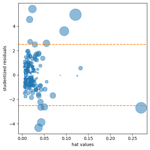

mask = [dist < 0.08 for dist in influence.cooks_distance[0]]
house_infl = house_98105.loc[mask]

ols_infl = sm.OLS(house_infl[outcome], sm.add_constant(house_infl[predictors]))
result_infl = ols_infl.fit()

pd.DataFrame({
    "Original": result_98105.params,
    "Influential removed": result_infl.params,
})

	Original	Influential removed
const	-772549.862447	-647137.096716
SqFtTotLiving	209.602346	230.052569
SqFtLot	38.933315	33.141600
Bathrooms	2282.264145	-16131.879785
Bedrooms	-26320.268796	-22887.865318
BldgGrade	130000.099737	114870.559737

Heteroskedasticity, Nonnormality, and Correlated Errors

fig, ax = plt.subplots(figsize=(5, 5))
sns.regplot(x=result_98105.fittedvalues, y=np.abs(result_98105.resid),
            scatter_kws={"alpha": 0.25}, line_kws={"color": "C1"},
            lowess=True, ax=ax)
ax.set_xlabel("predicted")
ax.set_ylabel("abs(residual)")

plt.tight_layout()
plt.show()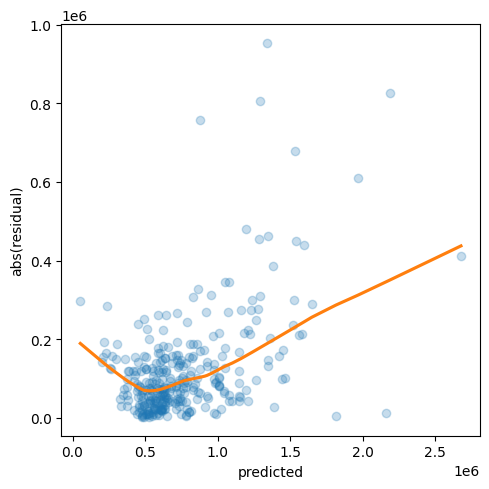

Partial Residual Plots and Nonlinearity

sm.graphics.plot_ccpr(result_98105, "SqFtTotLiving")

plt.tight_layout()
plt.show()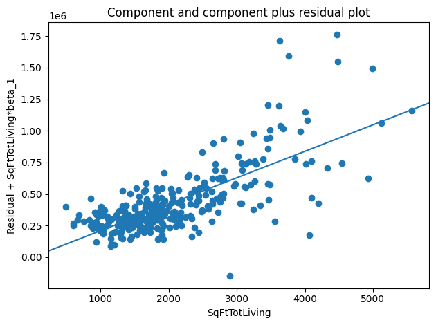

Polynomial and Spline Regression

Polynomial

model_poly = smf.ols(formula="AdjSalePrice ~  SqFtTotLiving + "
                "I(SqFtTotLiving**2) + "
                "SqFtLot + Bathrooms + Bedrooms + BldgGrade", data=house_98105)
result_poly = model_poly.fit()
result_poly.summary()

OLS Regression Results
Dep. Variable:	AdjSalePrice	R-squared:	0.806
Model:	OLS	Adj. R-squared:	0.802
Method:	Least Squares	F-statistic:	211.6
Date:	Tue, 09 Jun 2026	Prob (F-statistic):	9.95e-106
Time:	18:18:24	Log-Likelihood:	-4217.9
No. Observations:	313	AIC:	8450.
Df Residuals:	306	BIC:	8476.
Df Model:	6
Covariance Type:	nonrobust

	coef	std err	t	P>\|t\|	[0.025	0.975]
Intercept	-6.159e+05	1.03e+05	-5.953	0.000	-8.19e+05	-4.12e+05
SqFtTotLiving	7.4521	55.418	0.134	0.893	-101.597	116.501
I(SqFtTotLiving ** 2)	0.0388	0.010	4.040	0.000	0.020	0.058
SqFtLot	32.5594	5.436	5.990	0.000	21.863	43.256
Bathrooms	-1435.1231	1.95e+04	-0.074	0.941	-3.99e+04	3.7e+04
Bedrooms	-9191.9441	1.33e+04	-0.693	0.489	-3.53e+04	1.69e+04
BldgGrade	1.357e+05	1.49e+04	9.087	0.000	1.06e+05	1.65e+05

Omnibus:	75.161	Durbin-Watson:	1.625
Prob(Omnibus):	0.000	Jarque-Bera (JB):	637.978
Skew:	0.699	Prob(JB):	2.92e-139
Kurtosis:	9.853	Cond. No.	7.37e+07

Notes:
[1] Standard Errors assume that the covariance matrix of the errors is correctly specified.
[2] The condition number is large, 7.37e+07. This might indicate that there are
strong multicollinearity or other numerical problems.

Splines

formula = ("AdjSalePrice ~ bs(SqFtTotLiving, df=6, degree=3) + "
           "SqFtLot + Bathrooms + Bedrooms + BldgGrade")
model_spline = smf.ols(formula=formula, data=house_98105)
result_spline = model_spline.fit()

Generalized Additive Models

predictors = ["SqFtTotLiving", "SqFtLot", "Bathrooms", "Bedrooms", "BldgGrade"]
outcome = "AdjSalePrice"
X = house_98105[predictors].to_numpy()
y = house_98105[outcome]

gam = LinearGAM(s(0, n_splines=12) + l(1) + l(2) + l(3) + l(4))
gam.gridsearch(X, y)
print(gam.summary())

  0% (0 of 11) |                         | Elapsed Time: 0:00:00 ETA:  --:--:--

100% (11 of 11) |########################| Elapsed Time: 0:00:00 Time:  0:00:00

LinearGAM                                                                                                 
=============================================== ==========================================================
Distribution:                        NormalDist Effective DoF:                                      7.6772
Link Function:                     IdentityLink Log Likelihood:                                 -4213.0332
Number of Samples:                          313 AIC:                                             8443.4209
                                                AICc:                                            8443.9746
                                                GCV:                                      30838885095.1688
                                                Scale:                                         171698.5198
                                                Pseudo R-Squared:                                   0.8117
==========================================================================================================
Feature Function                  Lambda               Rank         EDoF         P > x        Sig. Code   
================================= ==================== ============ ============ ============ ============
s(0)                              [15.8489]            12           4.3          0.00e+00     ***         
l(1)                              [15.8489]            1            0.9          2.35e-10     ***         
l(2)                              [15.8489]            1            0.8          8.45e-01                 
l(3)                              [15.8489]            1            0.9          3.79e-01                 
l(4)                              [15.8489]            1            0.8          0.00e+00     ***         
intercept                                              1            0.0          9.14e-01                 
==========================================================================================================
Significance codes:  0 '***' 0.001 '**' 0.01 '*' 0.05 '.' 0.1 ' ' 1

WARNING: Fitting splines and a linear function to a feature introduces a model identifiability problem
         which can cause p-values to appear significant when they are not.

WARNING: p-values calculated in this manner behave correctly for un-penalized models or models with
         known smoothing parameters, but when smoothing parameters have been estimated, the p-values
         are typically lower than they should be, meaning that the tests reject the null too readily.
None

/var/folders/_8/ms0ft4913k3290v7f0g_yfpc0000gn/T/ipykernel_27334/4156786098.py:8: UserWarning: KNOWN BUG: p-values computed in this summary are likely much smaller than they should be. 
 
Please do not make inferences based on these values! 

Collaborate on a solution, and stay up to date at: 
github.com/dswah/pyGAM/issues/163 

  print(gam.summary())

Supplementary Material

Figure 4-1. Cotton exposure versus lung capacity

lung = pd.read_csv(DATA_DIR / "LungDisease.csv")

lung.plot.scatter(x="Exposure", y="PEFR")

plt.tight_layout()
plt.show()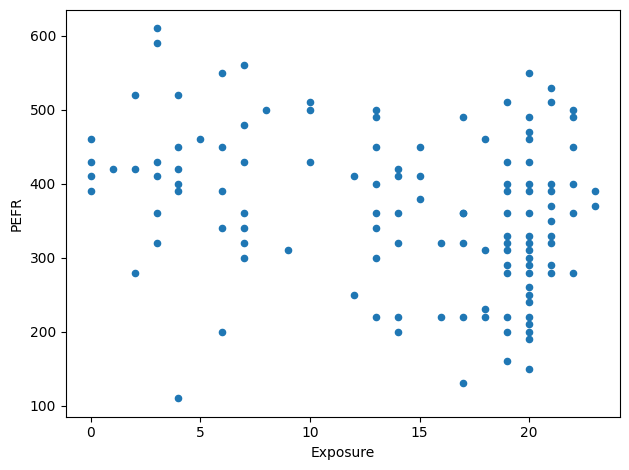

Figure 4-2. Slope and intercept for the regression fit to the lung data

predictors = ["Exposure"]
outcome = "PEFR"
model = LinearRegression()
model.fit(lung[predictors], lung[outcome])

fig, ax = plt.subplots(figsize=(4, 4))
ax.set_xlim(0, 23)
ax.set_ylim(295, 450)
ax.set_xlabel("Exposure")
ax.set_ylabel("PEFR")
ax.plot((0, 23), model.predict(pd.DataFrame({"Exposure": [0, 23]})))
ax.text(0.4, model.intercept_, r"$b_0$", size="larger")

x = pd.DataFrame({"Exposure": [7.5, 17.5]})
y = model.predict(x)
ax.plot((7.5, 7.5, 17.5), (y[0], y[1], y[1]), "--")
ax.text(5, np.mean(y), r"$\Delta Y$", size="larger")
ax.text(12, y[1] - 10, r"$\Delta X$", size="larger")
ax.text(12, 390, r"$b_1 = \frac{\Delta Y}{\Delta X}$", size="larger")

plt.tight_layout()
plt.show()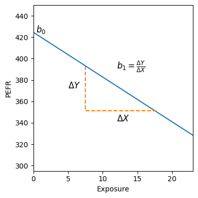

Figure 4-3. Residuals for the regression fit to the lung data

fitted = model.predict(lung[predictors])
residuals = lung[outcome] - fitted

ax = lung.plot.scatter(x="Exposure", y="PEFR", figsize=(4, 4), zorder=10)
ax.plot(lung.Exposure, fitted)
for x, yactual, yfitted in zip(lung.Exposure, lung.PEFR, fitted, strict=True):
    ax.plot((x, x), (yactual, yfitted), "--", color="C1")

plt.tight_layout()
plt.show()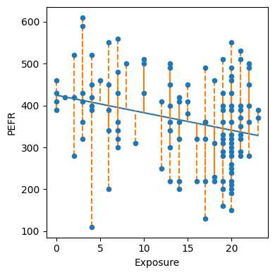

Figure 4-5. An example of an influential data point in regression

rng = np.random.default_rng(seed=5)
x = rng.normal(size=25)
y = -x / 5 + rng.normal(size=25)
x[0] = 8
y[0] = 8

def abline(slope, intercept, ax):
    """Calculate coordinates of a line based on slope and intercept"""
    x_vals = np.array(ax.get_xlim())
    return (x_vals, intercept + slope * x_vals)

fig, ax = plt.subplots(figsize=(4, 4))
ax.scatter(x, y)
slope, intercept, _, _, _ = linregress(x, y)
ax.plot(*abline(slope, intercept, ax))
slope, intercept, _, _, _ = linregress(x[1:], y[1:])
ax.plot(*abline(slope, intercept, ax), "--")
ax.set_xlim(-2.5, 8.5)
ax.set_ylim(-2.5, 8.5)

plt.tight_layout()
plt.show()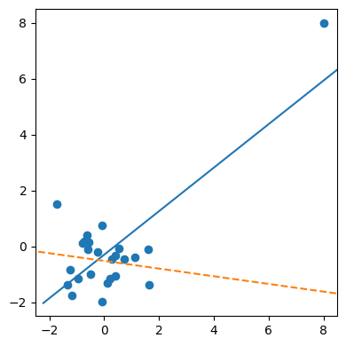

Figure 4-8. A histogram of the residuals from the regression of the housing data

fig, ax = plt.subplots(figsize=(4, 4))
pd.Series(influence.resid_studentized_internal).hist(ax=ax)
ax.set_xlabel("std. residual")
ax.set_ylabel("Frequency")

plt.tight_layout()
plt.show()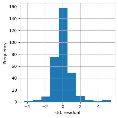

Figure 4-10. A polynomial regression fit for the variable SqFtTotLiving

(solid line) versus a smooth (dashed line; see the following section about splines)

def partial_residual_plot(model, df, outcome, feature, ax):
    y_pred = model.predict(df)
    # determine columns required for model
    required = set(model.params.index).intersection(df.columns)
    required.add(feature)
    # create a copy of df with only required columns and set everything
    # except the features to zero
    copy_df = df[list(required)].copy().astype("float")
    for c in copy_df.columns:
        if c == feature:
            continue
        copy_df.loc[:, c] = 0.0
    feature_prediction = model.predict(copy_df)
    results = pd.DataFrame({
        "feature": df[feature],
        "residual": df[outcome] - y_pred,
        "ypartial": feature_prediction - model.params.iloc[0],
    })
    results = results.sort_values(by=["feature"])
    smoothed = sm.nonparametric.lowess(results.ypartial + results.residual, results.feature,
        frac=1 / 3)

    ax.scatter(results.feature, results.ypartial + results.residual)
    ax.plot(smoothed[:, 0], smoothed[:, 1], color="gray")
    ax.plot(results.feature, results.ypartial, color="black")
    ax.set_xlabel(feature)
    ax.set_ylabel(f"Residual + {feature} contribution")
    return ax

fig, ax = plt.subplots(figsize=(5, 5))
partial_residual_plot(result_poly, house_98105, "AdjSalePrice", "SqFtTotLiving", ax)

plt.tight_layout()
plt.show()
print(result_poly.params.iloc[2])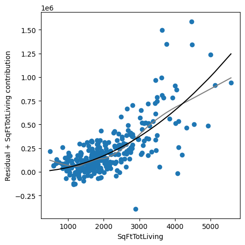

0.03879128168239703

Figure 4-12. A spline regression fit for the variable SqFtTotLiving (solid line) compared to a smooth (dashed line)

fig, ax = plt.subplots(figsize=(5, 5))
partial_residual_plot(result_spline, house_98105, "AdjSalePrice", "SqFtTotLiving", ax)

plt.tight_layout()
plt.show()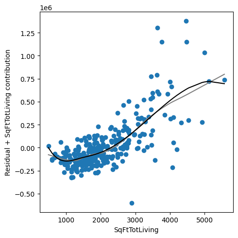

Figure 4-13. A GAM regression fit for the variable SqFtTotLiving (solid line) compared to a smooth (dashed line)

fig, axes = plt.subplots(figsize=(8, 8), ncols=2, nrows=3)

titles = ["SqFtTotLiving", "SqFtLot", "Bathrooms", "Bedrooms", "BldgGrade"]
for i, title in enumerate(titles):
    ax = axes[i // 2, i % 2]
    XX = gam.generate_X_grid(term=i)
    ax.plot(XX[:, i], gam.partial_dependence(term=i, X=XX))
    ax.plot(XX[:, i], gam.partial_dependence(term=i, X=XX, width=.95)[1], c="r", ls="--")
    ax.set_title(title)

axes[2][1].set_visible(False)

plt.tight_layout()
plt.show()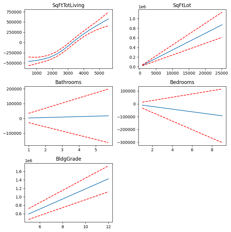

Generalized additive models using statsmodels

predictors = ["SqFtTotLiving", "SqFtLot", "Bathrooms", "Bedrooms", "BldgGrade"]
outcome = "AdjSalePrice"

x_spline = house_98105[predictors]
bs = BSplines(x_spline, df=[10] + [3] * 4, degree=[3] + [2] * 4)
# penalization weight
alpha = np.array([0] * 5)

formula = ("AdjSalePrice ~ SqFtTotLiving + "
           "SqFtLot + Bathrooms + Bedrooms + BldgGrade")

gam_sm = GLMGam.from_formula(formula, data=house_98105, smoother=bs, alpha=alpha)
res_sm = gam_sm.fit()
print(res_sm.summary())

                 Generalized Linear Model Regression Results                  
==============================================================================
Dep. Variable:           AdjSalePrice   No. Observations:                  313
Model:                         GLMGam   Df Residuals:                   295.00
Model Family:                Gaussian   Df Model:                        17.00
Link Function:               Identity   Scale:                      2.7471e+10
Method:                         PIRLS   Log-Likelihood:                -4196.6
Date:                Tue, 09 Jun 2026   Deviance:                   8.1039e+12
Time:                        18:18:24   Pearson chi2:                 8.10e+12
No. Iterations:                     3   Pseudo R-squ. (CS):             0.9901
Covariance Type:            nonrobust                                         
====================================================================================
                       coef    std err          z      P>|z|      [0.025      0.975]
------------------------------------------------------------------------------------
Intercept        -3.481e+05   1.18e+05     -2.962      0.003   -5.79e+05   -1.18e+05
SqFtTotLiving      192.1472     50.663      3.793      0.000      92.849     291.446
SqFtLot              6.9002      7.654      0.902      0.367      -8.101      21.902
Bathrooms        -7836.2808   2.12e+04     -0.370      0.712   -4.94e+04    3.37e+04
Bedrooms         -8297.4370   1.26e+04     -0.660      0.509   -3.29e+04    1.63e+04
BldgGrade         1.014e+05    1.4e+04      7.249      0.000     7.4e+04    1.29e+05
SqFtTotLiving_s0  1.465e+05   2.34e+05      0.626      0.531   -3.12e+05    6.05e+05
SqFtTotLiving_s1 -6.174e+04   1.33e+05     -0.464      0.642   -3.22e+05    1.99e+05
SqFtTotLiving_s2 -3.186e+04   1.26e+05     -0.253      0.800   -2.78e+05    2.15e+05
SqFtTotLiving_s3 -5.403e+04   1.01e+05     -0.535      0.593   -2.52e+05    1.44e+05
SqFtTotLiving_s4 -1.182e+05   1.01e+05     -1.167      0.243   -3.17e+05    8.03e+04
SqFtTotLiving_s5 -1.295e+05   8.23e+04     -1.574      0.115   -2.91e+05    3.17e+04
SqFtTotLiving_s6 -3.014e+04   1.27e+05     -0.237      0.813    -2.8e+05     2.2e+05
SqFtTotLiving_s7  1.262e+05    1.8e+05      0.702      0.483   -2.26e+05    4.79e+05
SqFtTotLiving_s8  5.325e+04   1.38e+05      0.386      0.700   -2.17e+05    3.24e+05
SqFtLot_s0        5.775e+05   1.58e+05      3.651      0.000    2.68e+05    8.88e+05
SqFtLot_s1       -2.771e+05   7.86e+04     -3.526      0.000   -4.31e+05   -1.23e+05
Bathrooms_s0      3.723e+04   1.06e+05      0.351      0.726   -1.71e+05    2.45e+05
Bathrooms_s1      5.303e+04   5.94e+04      0.892      0.372   -6.35e+04     1.7e+05
Bedrooms_s0       2.298e+05   1.31e+05      1.751      0.080   -2.74e+04    4.87e+05
Bedrooms_s1      -7.241e+04   6.81e+04     -1.063      0.288   -2.06e+05    6.11e+04
BldgGrade_s0     -7.953e+05   2.03e+05     -3.917      0.000   -1.19e+06   -3.97e+05
BldgGrade_s1      6.608e+05   1.14e+05      5.818      0.000    4.38e+05    8.83e+05
====================================================================================

res_sm.plot_partial(0, cpr=True)

plt.tight_layout()
plt.show()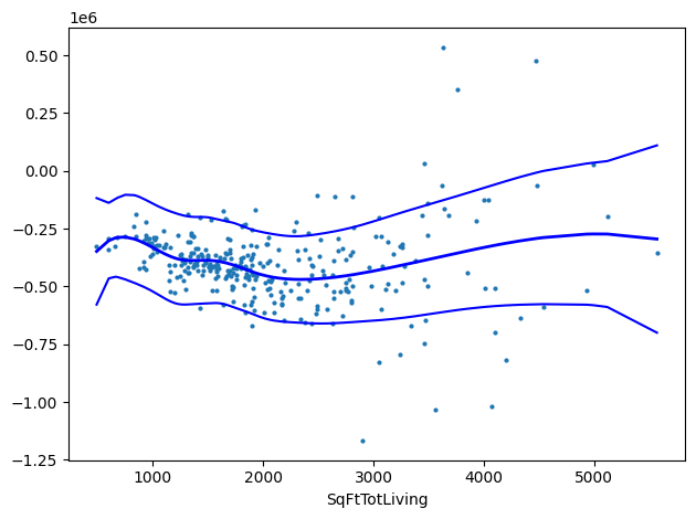

Additional material not covered in book

Regularization - Lasso

predictors = ["SqFtTotLiving", "SqFtLot", "Bathrooms", "Bedrooms",
              "BldgGrade", "PropertyType", "NbrLivingUnits",
              "SqFtFinBasement", "YrBuilt", "YrRenovated",
              "NewConstruction"]
outcome = "AdjSalePrice"

X = pd.get_dummies(house[predictors], drop_first=True)
X["NewConstruction"] = [1 if nc else 0 for nc in X["NewConstruction"]]
columns = X.columns
X = StandardScaler().fit_transform(X)
y = house[outcome]

house_lm = LinearRegression()
print(house_lm.fit(X, y))

LinearRegression()

house_lasso = Lasso(alpha=10)
print(house_lasso.fit(X, y))

Lasso(alpha=10)

Method = LassoLars
MethodCV = LassoLarsCV
Method = Lasso
MethodCV = LassoCV

alpha_values = []
results = []
for alpha in [0.001, 0.01, 0.1, 1, 10, 100, 1000, 10000, 100000, 1000000, 10000000]:
    model = Method(alpha=alpha)
    model.fit(X, y)
    alpha_values.append(alpha)
    results.append(model.coef_)
modelCV = MethodCV(cv=5)
modelCV.fit(X, y)
ax = pd.DataFrame(results, index=alpha_values, columns=columns).plot(logx=True, legend=False)
ax.axvline(modelCV.alpha_)
plt.show()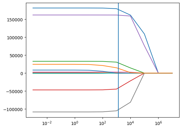

# Note that some of the coefficients are shrunk to zero
pd.DataFrame({
    "name": columns,
    "coef": modelCV.coef_,
})

	name	coef
0	SqFtTotLiving	178995.820585
1	SqFtLot	1110.585770
2	Bathrooms	29843.352268
3	Bedrooms	-43790.256319
4	BldgGrade	161882.297251
5	NbrLivingUnits	-0.000000
6	SqFtFinBasement	3248.457098
7	YrBuilt	-104164.720862
8	YrRenovated	0.000000
9	NewConstruction	-0.000000
10	PropertyType_Single Family	-0.000000
11	PropertyType_Townhouse	14255.932699

	fit_intercept fit_intercept: bool, default=True Whether to calculate the intercept for this model. If set to False, no intercept will be used in calculations (i.e. data is expected to be centered).	True
	copy_X copy_X: bool, default=True If True, X will be copied; else, it may be overwritten.	True
	tol tol: float, default=1e-6 The precision of the solution (`coef_`) is determined by `tol` which specifies a different convergence criterion for the `lsqr` solver. `tol` is set as `atol` and `btol` of :func:`scipy.sparse.linalg.lsqr` when fitting on sparse training data. This parameter has no effect when fitting on dense data. .. versionadded:: 1.7	1e-06
	n_jobs n_jobs: int, default=None The number of jobs to use for the computation. This will only provide speedup in case of sufficiently large problems, that is if firstly `n_targets > 1` and secondly `X` is sparse or if `positive` is set to `True`. ``None`` means 1 unless in a :obj:`joblib.parallel_backend` context. ``-1`` means using all processors. See :term:`Glossary ` for more details.	None
	positive positive: bool, default=False When set to ``True``, forces the coefficients to be positive. This option is only supported for dense arrays. For a comparison between a linear regression model with positive constraints on the regression coefficients and a linear regression without such constraints, see :ref:`sphx_glr_auto_examples_linear_model_plot_nnls.py`. .. versionadded:: 0.24	False

	steps steps: list of tuples List of (name of step, estimator) tuples that are to be chained in sequential order. To be compatible with the scikit-learn API, all steps must define `fit`. All non-last steps must also define `transform`. See :ref:`Combining Estimators ` for more details.	[('sfs', ...), ('model', ...)]
	transform_input transform_input: list of str, default=None The names of the :term:`metadata` parameters that should be transformed by the pipeline before passing it to the step consuming it. This enables transforming some input arguments to ``fit`` (other than ``X``) to be transformed by the steps of the pipeline up to the step which requires them. Requirement is defined via :ref:`metadata routing `. For instance, this can be used to pass a validation set through the pipeline. You can only set this if metadata routing is enabled, which you can enable using ``sklearn.set_config(enable_metadata_routing=True)``. .. versionadded:: 1.6	None
	memory memory: str or object with the joblib.Memory interface, default=None Used to cache the fitted transformers of the pipeline. The last step will never be cached, even if it is a transformer. By default, no caching is performed. If a string is given, it is the path to the caching directory. Enabling caching triggers a clone of the transformers before fitting. Therefore, the transformer instance given to the pipeline cannot be inspected directly. Use the attribute ``named_steps`` or ``steps`` to inspect estimators within the pipeline. Caching the transformers is advantageous when fitting is time consuming. See :ref:`sphx_glr_auto_examples_neighbors_plot_caching_nearest_neighbors.py` for an example on how to enable caching.	None
	verbose verbose: bool, default=False If True, the time elapsed while fitting each step will be printed as it is completed.	False

	fit_intercept fit_intercept: bool, default=True Whether to calculate the intercept for this model. If set to False, no intercept will be used in calculations (i.e. data is expected to be centered).	True
	copy_X copy_X: bool, default=True If True, X will be copied; else, it may be overwritten.	True
	tol tol: float, default=1e-6 The precision of the solution (`coef_`) is determined by `tol` which specifies a different convergence criterion for the `lsqr` solver. `tol` is set as `atol` and `btol` of :func:`scipy.sparse.linalg.lsqr` when fitting on sparse training data. This parameter has no effect when fitting on dense data. .. versionadded:: 1.7	1e-06
	n_jobs n_jobs: int, default=None The number of jobs to use for the computation. This will only provide speedup in case of sufficiently large problems, that is if firstly `n_targets > 1` and secondly `X` is sparse or if `positive` is set to `True`. ``None`` means 1 unless in a :obj:`joblib.parallel_backend` context. ``-1`` means using all processors. See :term:`Glossary ` for more details.	None
	positive positive: bool, default=False When set to ``True``, forces the coefficients to be positive. This option is only supported for dense arrays. For a comparison between a linear regression model with positive constraints on the regression coefficients and a linear regression without such constraints, see :ref:`sphx_glr_auto_examples_linear_model_plot_nnls.py`. .. versionadded:: 0.24	False

	fit_intercept fit_intercept: bool, default=True Whether to calculate the intercept for this model. If set to False, no intercept will be used in calculations (i.e. data is expected to be centered).	True
	copy_X copy_X: bool, default=True If True, X will be copied; else, it may be overwritten.	True
	tol tol: float, default=1e-6 The precision of the solution (`coef_`) is determined by `tol` which specifies a different convergence criterion for the `lsqr` solver. `tol` is set as `atol` and `btol` of :func:`scipy.sparse.linalg.lsqr` when fitting on sparse training data. This parameter has no effect when fitting on dense data. .. versionadded:: 1.7	1e-06
	n_jobs n_jobs: int, default=None The number of jobs to use for the computation. This will only provide speedup in case of sufficiently large problems, that is if firstly `n_targets > 1` and secondly `X` is sparse or if `positive` is set to `True`. ``None`` means 1 unless in a :obj:`joblib.parallel_backend` context. ``-1`` means using all processors. See :term:`Glossary ` for more details.	None
	positive positive: bool, default=False When set to ``True``, forces the coefficients to be positive. This option is only supported for dense arrays. For a comparison between a linear regression model with positive constraints on the regression coefficients and a linear regression without such constraints, see :ref:`sphx_glr_auto_examples_linear_model_plot_nnls.py`. .. versionadded:: 0.24	False

	fit_intercept fit_intercept: bool, default=True Whether to calculate the intercept for this model. If set to False, no intercept will be used in calculations (i.e. data is expected to be centered).	True
	copy_X copy_X: bool, default=True If True, X will be copied; else, it may be overwritten.	True
	tol tol: float, default=1e-6 The precision of the solution (`coef_`) is determined by `tol` which specifies a different convergence criterion for the `lsqr` solver. `tol` is set as `atol` and `btol` of :func:`scipy.sparse.linalg.lsqr` when fitting on sparse training data. This parameter has no effect when fitting on dense data. .. versionadded:: 1.7	1e-06
	n_jobs n_jobs: int, default=None The number of jobs to use for the computation. This will only provide speedup in case of sufficiently large problems, that is if firstly `n_targets > 1` and secondly `X` is sparse or if `positive` is set to `True`. ``None`` means 1 unless in a :obj:`joblib.parallel_backend` context. ``-1`` means using all processors. See :term:`Glossary ` for more details.	None
	positive positive: bool, default=False When set to ``True``, forces the coefficients to be positive. This option is only supported for dense arrays. For a comparison between a linear regression model with positive constraints on the regression coefficients and a linear regression without such constraints, see :ref:`sphx_glr_auto_examples_linear_model_plot_nnls.py`. .. versionadded:: 0.24	False

	estimator	LinearRegression()
	k_features	(1, ...)
	forward	False
	floating	True
	verbose	0
	scoring	'neg_root_mean_squared_error'
	cv	5
	n_jobs	-1
	pre_dispatch	'2*n_jobs'
	clone_estimator	True
	fixed_features	None
	feature_groups	None