Chapter 5: Classification

2019-2026 Peter C. Bruce, Andrew Bruce, Peter Gedeck

# from statsmodels.genmod.generalized_linear_model import GLMResults
from imblearn.over_sampling import SMOTE, ADASYN
from sklearn.compose import ColumnTransformer
from sklearn.discriminant_analysis import LinearDiscriminantAnalysis
from sklearn.linear_model import LogisticRegression
from sklearn.metrics import confusion_matrix
from sklearn.metrics import precision_score, recall_score
from sklearn.metrics import roc_auc_score
from sklearn.metrics import roc_curve
from sklearn.naive_bayes import MultinomialNB
from sklearn.pipeline import Pipeline
from sklearn.preprocessing import OneHotEncoder, KBinsDiscretizer
from sklearn.preprocessing import OrdinalEncoder
from sklearn.tree import DecisionTreeClassifier
import matplotlib.pyplot as plt
import mlba
import numpy as np
import pandas as pd
import pygam
import random
import seaborn as sns
import statsmodels.api as sm
import statsmodels.formula.api as smf

random.seed(123)

# Location of the data files. Adjust this path if you keep the data
# files in a different directory.
from pathlib import Path
DATA_DIR = Path('../data')

Classification

Naive Bayes

The Naive Solution

loan_data = pd.read_csv(DATA_DIR / "loan_data.csv.gz")

predictors = ["purpose_", "home_", "emp_len_"]
outcome = "outcome"
X = pd.get_dummies(loan_data[predictors], prefix="", prefix_sep="", dtype=int)
y = loan_data[outcome]

naive_model = MultinomialNB(alpha=0.01, fit_prior=True)
naive_model.fit(X, y)

MultinomialNB(alpha=0.01)

In a Jupyter environment, please rerun this cell to show the HTML representation or trust the notebook.
On GitHub, the HTML representation is unable to render, please try loading this page with nbviewer.org.

new_loan = X.loc[146:146, :]

print("predicted class: ", naive_model.predict(new_loan)[0])

probabilities = pd.DataFrame(naive_model.predict_proba(new_loan),
                             columns=naive_model.classes_)
print("predicted probabilities", probabilities)

predicted class:  default
predicted probabilities     default  paid off
0  0.653696  0.346304

Numeric Predictor Variables

num_cols = ["borrower_score", "payment_inc_ratio"]
cat_cols = ["purpose_", "home_", "emp_len_"]
mixed_naive_model = Pipeline([
    ("pre", ColumnTransformer([
        ("cat", OneHotEncoder(handle_unknown="ignore"), cat_cols),
        ("num", KBinsDiscretizer(n_bins=5, strategy="uniform"), num_cols),
    ])),
    ("clf", MultinomialNB()),
])
X = loan_data[cat_cols + num_cols]
mixed_naive_model.fit(X, loan_data["outcome"])

Pipeline(steps=[('pre',
                 ColumnTransformer(transformers=[('cat',
                                                  OneHotEncoder(handle_unknown='ignore'),
                                                  ['purpose_', 'home_',
                                                   'emp_len_']),
                                                 ('num',
                                                  KBinsDiscretizer(strategy='uniform'),
                                                  ['borrower_score',
                                                   'payment_inc_ratio'])])),
                ('clf', MultinomialNB())])

Discriminant Analysis

A Simple Example

loan3000 = pd.read_csv(DATA_DIR / "loan3000.csv")

loan3000.outcome = loan3000.outcome.astype("category")

predictors = ["borrower_score", "payment_inc_ratio"]
outcome = "outcome"

X = loan3000[predictors]
y = loan3000[outcome]

loan_lda = LinearDiscriminantAnalysis()
loan_lda.fit(X, y)
pd.DataFrame(loan_lda.scalings_, index=X.columns)

	0
borrower_score	7.175839
payment_inc_ratio	-0.099676

pred = pd.DataFrame(loan_lda.predict_proba(loan3000[predictors]),
                    columns=loan_lda.classes_)
pred.head()

	default	paid off
0	0.553544	0.446456
1	0.558953	0.441047
2	0.272696	0.727304
3	0.506254	0.493746
4	0.609952	0.390048

# Use scalings and center of means to determine decision boundary
center = np.mean(loan_lda.means_, axis=0)
slope = - loan_lda.scalings_[0] / loan_lda.scalings_[1]
intercept = center[1] - center[0] * slope

# payment_inc_ratio for borrower_score of 0 and 20
x_0 = (0 - intercept) / slope
x_20 = (20 - intercept) / slope

lda_df = pd.concat([loan3000, pred["default"]], axis=1)
lda_df.head()

fig, ax = plt.subplots(figsize=(4, 4))
g = sns.scatterplot(x="borrower_score", y="payment_inc_ratio",
                    hue="default", data=lda_df,
                    palette=sns.diverging_palette(240, 10, n=9, as_cmap=True),
                    ax=ax, legend=False)

ax.set_ylim(0, 20)
ax.set_xlim(0.15, 0.8)
ax.plot((x_0, x_20), (0, 20), linewidth=3)
ax.plot(*loan_lda.means_.transpose())

plt.tight_layout()
plt.show()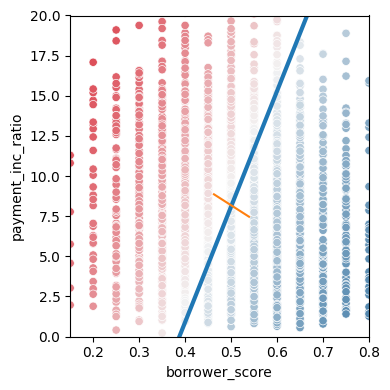

Logistic Regression

Logistic Regression and the GLM

predictors = ["payment_inc_ratio", "purpose_", "home_", "emp_len_",
              "borrower_score"]
outcome = "outcome"
X = pd.get_dummies(loan_data[predictors], prefix="", prefix_sep="",
                   drop_first=True, dtype=int)
y = loan_data[outcome]

logit_reg = LogisticRegression(C=np.inf, max_iter=1000)
logit_reg.fit(X, y)

/Users/petergedeck/cdd/practical-statistics-for-data-scientists-code-3e/.venv/lib/python3.13/site-packages/sklearn/linear_model/_logistic.py:1170: UserWarning: Setting penalty=None will ignore the C and l1_ratio parameters
  warnings.warn(

LogisticRegression(C=inf, max_iter=1000)

print("intercept ", logit_reg.intercept_[0])
print("classes", logit_reg.classes_)
pd.DataFrame({"coeff": logit_reg.coef_[0]}, index=X.columns)

intercept  -1.6261242575653818
classes ['default' 'paid off']

	coeff
payment_inc_ratio	-0.079885
borrower_score	4.610744
debt_consolidation	-0.250128
home_improvement	-0.411826
major_purchase	-0.228901
medical	-0.528521
other	-0.620839
small_business	-1.222285
OWN	-0.052460
RENT	-0.159205
> 1 Year	0.349254

Predicted Values from Logistic Regression

pred = pd.DataFrame(logit_reg.predict_log_proba(X),
                    columns=logit_reg.classes_)
pred.describe()

	default	paid off
count	45342.000000	45342.000000
mean	-0.758078	-0.760365
std	0.378317	0.390689
min	-2.771842	-3.546430
25%	-0.986107	-0.977608
50%	-0.697477	-0.688836
75%	-0.471941	-0.466850
max	-0.029251	-0.064588

pred = pd.DataFrame(logit_reg.predict_proba(X),
                    columns=logit_reg.classes_)
pred.describe()

	default	paid off
count	45342.000000	45342.000000
mean	0.499934	0.500066
std	0.167427	0.167427
min	0.062547	0.028827
25%	0.373026	0.376210
50%	0.497840	0.502160
75%	0.623790	0.626974
max	0.971173	0.937453

Assessing the Model

y_numbers = [1 if yi == "default" else 0 for yi in y]
logit_reg_sm = sm.GLM(y_numbers, X.assign(const=1),
                      family=sm.families.Binomial())
logit_result = logit_reg_sm.fit()
print(logit_result.summary())

                 Generalized Linear Model Regression Results                  
==============================================================================
Dep. Variable:                      y   No. Observations:                45342
Model:                            GLM   Df Residuals:                    45330
Model Family:                Binomial   Df Model:                           11
Link Function:                  Logit   Scale:                          1.0000
Method:                          IRLS   Log-Likelihood:                -28757.
Date:                Sun, 31 May 2026   Deviance:                       57515.
Time:                        18:07:11   Pearson chi2:                 4.54e+04
No. Iterations:                     4   Pseudo R-squ. (CS):             0.1112
Covariance Type:            nonrobust                                         
======================================================================================
                         coef    std err          z      P>|z|      [0.025      0.975]
--------------------------------------------------------------------------------------
payment_inc_ratio      0.0797      0.002     32.058      0.000       0.075       0.085
borrower_score        -4.6126      0.084    -55.203      0.000      -4.776      -4.449
debt_consolidation     0.2494      0.028      9.030      0.000       0.195       0.303
home_improvement       0.4077      0.047      8.747      0.000       0.316       0.499
major_purchase         0.2296      0.054      4.277      0.000       0.124       0.335
medical                0.5105      0.087      5.882      0.000       0.340       0.681
other                  0.6207      0.039     15.738      0.000       0.543       0.698
small_business         1.2153      0.063     19.192      0.000       1.091       1.339
OWN                    0.0483      0.038      1.271      0.204      -0.026       0.123
RENT                   0.1573      0.021      7.420      0.000       0.116       0.199
 > 1 Year             -0.3567      0.053     -6.779      0.000      -0.460      -0.254
const                  1.6381      0.074     22.224      0.000       1.494       1.783
======================================================================================

formula = ("outcome ~ bs(payment_inc_ratio, df=4) + purpose_ + "
           "home_ + emp_len_ + bs(borrower_score, df=4)")
model = smf.glm(formula=formula, data=loan_data, family=sm.families.Binomial())
results = model.fit()

print(results.summary())

                             Generalized Linear Model Regression Results                             
=====================================================================================================
Dep. Variable:     ['outcome[default]', 'outcome[paid off]']   No. Observations:                45342
Model:                                                   GLM   Df Residuals:                    45324
Model Family:                                       Binomial   Df Model:                           17
Link Function:                                         Logit   Scale:                          1.0000
Method:                                                 IRLS   Log-Likelihood:                -28744.
Date:                                       Sun, 31 May 2026   Deviance:                       57487.
Time:                                               18:07:11   Pearson chi2:                 4.54e+04
No. Iterations:                                            5   Pseudo R-squ. (CS):             0.1117
Covariance Type:                                   nonrobust                                         
==================================================================================================
                                     coef    std err          z      P>|z|      [0.025      0.975]
--------------------------------------------------------------------------------------------------
Intercept                          1.8382      0.380      4.836      0.000       1.093       2.583
purpose_[T.debt_consolidation]     0.2491      0.028      9.020      0.000       0.195       0.303
purpose_[T.home_improvement]       0.4138      0.047      8.848      0.000       0.322       0.505
purpose_[T.major_purchase]         0.2401      0.054      4.450      0.000       0.134       0.346
purpose_[T.medical]                0.5183      0.087      5.953      0.000       0.348       0.689
purpose_[T.other]                  0.6295      0.040     15.812      0.000       0.552       0.708
purpose_[T.small_business]         1.2252      0.063     19.303      0.000       1.101       1.350
home_[T.OWN]                       0.0484      0.038      1.273      0.203      -0.026       0.123
home_[T.RENT]                      0.1581      0.021      7.456      0.000       0.117       0.200
emp_len_[T. > 1 Year]             -0.3541      0.053     -6.729      0.000      -0.457      -0.251
bs(payment_inc_ratio, df=4)[0]     0.0049      0.121      0.041      0.967      -0.232       0.241
bs(payment_inc_ratio, df=4)[1]     1.6033      0.142     11.289      0.000       1.325       1.882
bs(payment_inc_ratio, df=4)[2]     1.9033      0.488      3.900      0.000       0.947       2.860
bs(payment_inc_ratio, df=4)[3]    -0.8521      1.929     -0.442      0.659      -4.633       2.929
bs(borrower_score, df=4)[0]       -1.0045      0.476     -2.112      0.035      -1.937      -0.072
bs(borrower_score, df=4)[1]       -2.6411      0.287     -9.209      0.000      -3.203      -2.079
bs(borrower_score, df=4)[2]       -3.6984      0.473     -7.824      0.000      -4.625      -2.772
bs(borrower_score, df=4)[3]       -5.8564      0.525    -11.160      0.000      -6.885      -4.828
==================================================================================================

Analysis of residuals

Evaluating Classification Models

Confusion Matrix

pred = logit_reg.predict(X)
pred_y = logit_reg.predict(X) == "default"
true_y = y == "default"
true_pos = true_y & pred_y
true_neg = ~true_y & ~pred_y
false_pos = ~true_y & pred_y
false_neg = true_y & ~pred_y

conf_mat = pd.DataFrame([[np.sum(true_pos), np.sum(false_neg)],
                         [np.sum(false_pos), np.sum(true_neg)]],
                       index=["Y = default", "Y = paid off"],
                       columns=["Yhat = default", "Yhat = paid off"])
conf_mat

	Yhat = default	Yhat = paid off
Y = default	14321	8350
Y = paid off	8140	14531

print(confusion_matrix(y_true=y, y_pred=logit_reg.predict(X)))

[[14321  8350]
 [ 8140 14531]]

mlba.classificationSummary(y_true=y, y_pred=logit_reg.predict(X))

Confusion Matrix (Accuracy 0.6363)

         Prediction
  Actual  default paid off
 default    14321     8350
paid off     8140    14531

Precision, Recall, and Specificity

y_pred = logit_reg.predict(X)
print("precision ", precision_score(y, y_pred, pos_label="default"))
print("recall.    ", recall_score(y, y_pred, pos_label="default"))
print("specificity", recall_score(y, y_pred, pos_label="paid off"))

precision  0.6375940519122034
recall.     0.6316880596356579
specificity 0.640950994662785

ROC Curve

fpr, tpr, thresholds = roc_curve(y, logit_reg.predict_proba(X)[:, 0],
                                 pos_label="default")
roc_df = pd.DataFrame({"recall": tpr, "specificity": 1 - fpr})

ax = roc_df.plot(x="specificity", y="recall", figsize=(4, 4), legend=False)
ax.set_ylim(0, 1)
ax.set_xlim(1, 0)
ax.plot((1, 0), (0, 1))
ax.set_xlabel("specificity")
ax.set_ylabel("recall")

plt.tight_layout()
plt.show()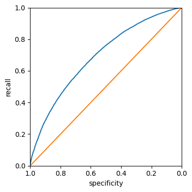

AUC

print(np.sum(roc_df.recall[:-1] * np.diff(1 - roc_df.specificity)))
print(roc_auc_score([1 if yi == "default" else 0 for yi in y],
                    logit_reg.predict_proba(X)[:, 0]))

0.6917057288869074
0.6917058067118191

Strategies for Imbalanced Data

Undersampling

full_train_set = pd.read_csv(DATA_DIR / "full_train_set.csv.gz")

print("percentage of loans in default: ",
      100 * np.mean(full_train_set.outcome == "default"))

percentage of loans in default:  18.894546909248504

predictors = ["payment_inc_ratio", "purpose_", "home_", "emp_len_",
              "dti", "revol_bal", "revol_util"]
outcome = "outcome"
X = pd.get_dummies(full_train_set[predictors], prefix="", prefix_sep="",
                   drop_first=True, dtype=int)
y = full_train_set[outcome]

full_model = LogisticRegression(C=np.inf, max_iter=10_000)
full_model.fit(X, y)
print("percentage of loans predicted to default: ",
      100 * np.mean(full_model.predict(X) == "default"))

/Users/petergedeck/cdd/practical-statistics-for-data-scientists-code-3e/.venv/lib/python3.13/site-packages/sklearn/linear_model/_logistic.py:1170: UserWarning: Setting penalty=None will ignore the C and l1_ratio parameters
  warnings.warn(

percentage of loans predicted to default:  0.3883754073357947

Oversampling and Up/Down Weighting

default_wt = 1 / np.mean(full_train_set.outcome == "default")
wt = [default_wt if outcome == "default" else 1
      for outcome in full_train_set.outcome]

full_model = LogisticRegression(C=np.inf, max_iter=10_000)
full_model.fit(X, y, sample_weight=wt)
print("percentage of loans predicted to default (weighting): ",
      100 * np.mean(full_model.predict(X) == "default"))

/Users/petergedeck/cdd/practical-statistics-for-data-scientists-code-3e/.venv/lib/python3.13/site-packages/sklearn/linear_model/_logistic.py:1170: UserWarning: Setting penalty=None will ignore the C and l1_ratio parameters
  warnings.warn(

percentage of loans predicted to default (weighting):  57.61874203038663

Supplementary Material

Figure 5-2. Graph of the logit function that maps a probability to a scale suitable for a linear model

p = np.arange(0.01, 1, 0.01)
df = pd.DataFrame({
    "p": p,
    "logit": np.log(p / (1 - p)),
    "odds": p / (1 - p),
})

fig, ax = plt.subplots(figsize=(3, 3))
ax.axhline(0, color="grey", linestyle="--")
ax.axvline(0.5, color="grey", linestyle="--")
ax.plot(df["p"], df["logit"])
ax.set_xlabel("Probability")
ax.set_ylabel("logit(p)")

plt.tight_layout()
plt.show()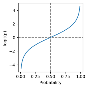

How to control the order of the classes in Python

# If you have a feature or outcome variable that is ordinal, use
# the scikit-learn `OrdinalEncoder` to replace the categories
# (here, "paid off" and "default") with numbers. In the below code,
# we replace "paid off" with 0 and "default" with 1. This reverses
# the order of the predicted classes and as a consequence, the
# coefficients will be reversed. You will however now need to
# keep track of how the the numbers map back to the classes.

predictors = ["payment_inc_ratio", "purpose_", "home_", "emp_len_",
              "borrower_score"]
outcome = "outcome"
X = pd.get_dummies(loan_data[predictors], prefix="", prefix_sep="",
                   drop_first=True, dtype=int)
enc = OrdinalEncoder(categories=[["paid off", "default"]])
y_enc = enc.fit_transform(loan_data[[outcome]]).ravel()

logit_reg_enc = LogisticRegression(C=np.inf, max_iter=1000)
logit_reg_enc.fit(X, y_enc)

print("intercept ", logit_reg_enc.intercept_[0])
print("classes", logit_reg_enc.classes_)
pd.DataFrame({"coeff": logit_reg_enc.coef_[0]}, index=X.columns)

intercept  1.6262802328204813
classes [0. 1.]

/Users/petergedeck/cdd/practical-statistics-for-data-scientists-code-3e/.venv/lib/python3.13/site-packages/sklearn/linear_model/_logistic.py:1170: UserWarning: Setting penalty=None will ignore the C and l1_ratio parameters
  warnings.warn(

	coeff
payment_inc_ratio	0.079896
borrower_score	-4.611003
debt_consolidation	0.250206
home_improvement	0.411879
major_purchase	0.228987
medical	0.528678
other	0.620869
small_business	1.222274
OWN	0.052453
RENT	0.159220
> 1 Year	-0.349459

Figure 5-3. The relationship between the odds ratio and the log-odds ratio

fig, ax = plt.subplots(figsize=(3, 3))
ax.plot(df["logit"], df["odds"])
ax.set_xlabel("log(odds ratio)")
ax.set_ylabel("odds ratio")
ax.set_xlim(0, 5.1)
ax.set_ylim(-5, 105)

plt.tight_layout()
plt.show()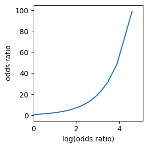

Figure 5-4. Partial residuals from logistic regression

def partial_residual_plot(model, df, outcome, feature, fig, ax):
    y_actual = [0 if s == "default" else 1 for s in df[outcome]]
    y_pred = model.predict(df)
    org_params = model.params.copy()
    zero_params = model.params.copy()
    # set model parametes of other features to 0
    for i, name in enumerate(zero_params.index):
        if feature in name:
            continue
        zero_params.iloc[i] = 0.0
    model.initialize(model.model, zero_params)
    feature_prediction = model.predict(df)
    ypartial = -np.log(1 / feature_prediction - 1)
    ypartial -= np.mean(ypartial)
    model.initialize(model.model, org_params)
    results = pd.DataFrame({
        "feature": df[feature],
        "residual": -2 * (y_actual - y_pred),
        "ypartial": ypartial / 2,
    })
    results = results.sort_values(by=["feature"])

    ax.scatter(results.feature, results.residual, marker=".", s=72. / fig.dpi)
    ax.plot(results.feature, results.ypartial, color="black")
    ax.set_xlabel(feature)
    ax.set_ylabel(f"Residual + {feature} contribution")
    return ax

formula = ("outcome ~ bs(payment_inc_ratio, df=8) + purpose_ + "
           "home_ + emp_len_ + bs(borrower_score, df=3)")
model = smf.glm(formula=formula, data=loan_data, family=sm.families.Binomial())
results = model.fit()

fig, ax = plt.subplots(figsize=(5, 5))
partial_residual_plot(results, loan_data, "outcome", "payment_inc_ratio", fig, ax)
ax.set_xlim(0, 25)
ax.set_ylim(-2.5, 2.5)


plt.tight_layout()
plt.show()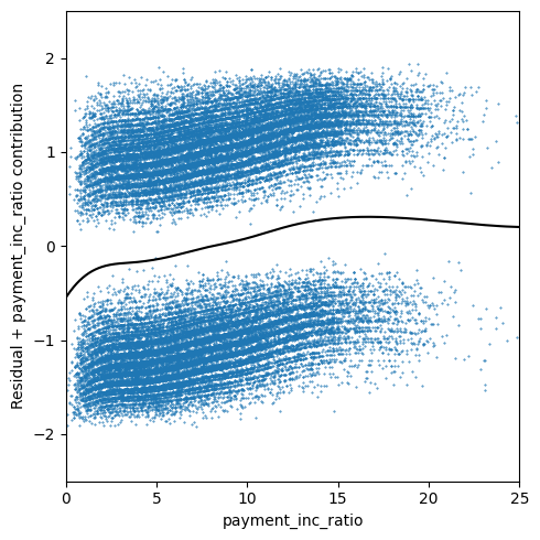

Figure 5-7. Area under the ROC curve for the loan data

ax = roc_df.plot(x="specificity", y="recall", figsize=(4, 4), legend=False)
ax.set_ylim(0, 1)
ax.set_xlim(1, 0)
ax.set_xlabel("specificity")
ax.set_ylabel("recall")
ax.fill_between(roc_df.specificity, 0, roc_df.recall, alpha=0.3)

plt.tight_layout()
plt.show()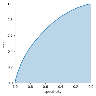

SMOTE

predictors = ["payment_inc_ratio", "purpose_", "home_", "emp_len_",
              "dti", "revol_bal", "revol_util"]
outcome = "outcome"
X = pd.get_dummies(full_train_set[predictors], prefix="", prefix_sep="",
                   drop_first=True, dtype=int)
y = full_train_set[outcome]

X_resampled, y_resampled = SMOTE().fit_resample(X, y)
print("percentage of loans in default (SMOTE resampled): ",
      f"{100 * np.mean(y_resampled == 'default'):.2f}")

full_model = LogisticRegression(C=np.inf, max_iter=10_000)
full_model.fit(X_resampled, y_resampled)
print("percentage of loans predicted to default (SMOTE): ",
      f"{100 * np.mean(full_model.predict(X) == 'default'):.2f}")

X_resampled, y_resampled = ADASYN().fit_resample(X, y)
print("percentage of loans in default (ADASYN resampled): ",
      f"{100 * np.mean(y_resampled == 'default'):.2f}")

full_model = LogisticRegression(C=np.inf, max_iter=10_000)
full_model.fit(X_resampled, y_resampled)
print("percentage of loans predicted to default (ADASYN): ",
      f"{100 * np.mean(full_model.predict(X) == 'default'):.2f}")

percentage of loans in default (SMOTE resampled):  50.00

/Users/petergedeck/cdd/practical-statistics-for-data-scientists-code-3e/.venv/lib/python3.13/site-packages/sklearn/linear_model/_logistic.py:1170: UserWarning: Setting penalty=None will ignore the C and l1_ratio parameters
  warnings.warn(

percentage of loans predicted to default (SMOTE):  29.51
percentage of loans in default (ADASYN resampled):  48.56

/Users/petergedeck/cdd/practical-statistics-for-data-scientists-code-3e/.venv/lib/python3.13/site-packages/sklearn/linear_model/_logistic.py:1170: UserWarning: Setting penalty=None will ignore the C and l1_ratio parameters
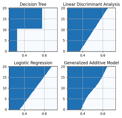
  warnings.warn(

percentage of loans predicted to default (ADASYN):  27.37

Figure 5-8. Comparison of the classification rules for four different methods

predictors = ["borrower_score", "payment_inc_ratio"]
outcome = "outcome"
X = loan3000[predictors]
y = loan3000[outcome]

loan_tree = DecisionTreeClassifier(random_state=1, criterion="entropy",
                                   min_impurity_decrease=0.003)
loan_tree.fit(X, y)

loan_lda = LinearDiscriminantAnalysis()
loan_lda.fit(X, y)

logit_reg = LogisticRegression(penalty="l2", solver="liblinear")
logit_reg.fit(X, y)


## model
gam = pygam.LinearGAM(pygam.s(0) + pygam.s(1))
print(gam.gridsearch(X.values, [1 if yi == "default" else 0 for yi in y]))

/Users/petergedeck/cdd/practical-statistics-for-data-scientists-code-3e/.venv/lib/python3.13/site-packages/sklearn/linear_model/_logistic.py:1135: FutureWarning: 'penalty' was deprecated in version 1.8 and will be removed in 1.10. To avoid this warning, leave 'penalty' set to its default value and use 'l1_ratio' or 'C' instead. Use l1_ratio=0 instead of penalty='l2', l1_ratio=1 instead of penalty='l1', and C=np.inf instead of penalty=None.

  warnings.warn(


  0% (0 of 11) |                         | Elapsed Time: 0:00:00 ETA:  --:--:--

 45% (5 of 11) |###########              | Elapsed Time: 0:00:00 ETA:   0:00:00

 90% (10 of 11) |#####################   | Elapsed Time: 0:00:00 ETA:   0:00:00

100% (11 of 11) |########################| Elapsed Time: 0:00:00 Time:  0:00:00

LinearGAM(callbacks=[Deviance(), Diffs()], fit_intercept=True, 
   max_iter=100, scale=None, terms=s(0) + s(1) + intercept, 
   tol=0.0001, verbose=False)

models = {
    "Decision Tree": loan_tree,
    "Linear Discriminant Analysis": loan_lda,
    "Logistic Regression": logit_reg,
    "Generalized Additive Model": gam,
}

fig, axes = plt.subplots(nrows=2, ncols=2, figsize=(5, 5))

xvalues = np.arange(0.25, 0.73, 0.005)
yvalues = np.arange(-0.1, 20.1, 0.1)
xx, yy = np.meshgrid(xvalues, yvalues)
X = pd.DataFrame({
    "borrower_score": xx.ravel(),
    "payment_inc_ratio": yy.ravel(),
})

boundary = {}

for n, (title, model) in enumerate(models.items()):
    ax = axes[n // 2, n % 2]
    predict = model.predict(X)
    if "Generalized" in title:
        Z = np.array([1 if z > 0.5 else 0 for z in predict])
    else:
        Z = np.array([1 if z == "default" else 0 for z in predict])
    Z = Z.reshape(xx.shape)
    boundary[title] = yvalues[np.argmax(Z > 0, axis=0)]
    boundary[title][Z[-1, :] == 0] = yvalues[-1]

    c = ax.pcolormesh(xx, yy, Z, cmap="Blues", vmin=0.1, vmax=1.3, shading="auto")
    ax.set_title(title)
    ax.grid(visible=True)

plt.tight_layout()
plt.show()

Naive Bayes with numerical features

print(f”MixedNB Library Accuracy: {accuracy_mixed:.2f}“)

	steps steps: list of tuples List of (name of step, estimator) tuples that are to be chained in sequential order. To be compatible with the scikit-learn API, all steps must define `fit`. All non-last steps must also define `transform`. See :ref:`Combining Estimators ` for more details.	[('pre', ...), ('clf', ...)]
	transform_input transform_input: list of str, default=None The names of the :term:`metadata` parameters that should be transformed by the pipeline before passing it to the step consuming it. This enables transforming some input arguments to ``fit`` (other than ``X``) to be transformed by the steps of the pipeline up to the step which requires them. Requirement is defined via :ref:`metadata routing `. For instance, this can be used to pass a validation set through the pipeline. You can only set this if metadata routing is enabled, which you can enable using ``sklearn.set_config(enable_metadata_routing=True)``. .. versionadded:: 1.6	None
	memory memory: str or object with the joblib.Memory interface, default=None Used to cache the fitted transformers of the pipeline. The last step will never be cached, even if it is a transformer. By default, no caching is performed. If a string is given, it is the path to the caching directory. Enabling caching triggers a clone of the transformers before fitting. Therefore, the transformer instance given to the pipeline cannot be inspected directly. Use the attribute ``named_steps`` or ``steps`` to inspect estimators within the pipeline. Caching the transformers is advantageous when fitting is time consuming. See :ref:`sphx_glr_auto_examples_neighbors_plot_caching_nearest_neighbors.py` for an example on how to enable caching.	None
	verbose verbose: bool, default=False If True, the time elapsed while fitting each step will be printed as it is completed.	False

	transformers transformers: list of tuples List of (name, transformer, columns) tuples specifying the transformer objects to be applied to subsets of the data. name : str Like in Pipeline and FeatureUnion, this allows the transformer and its parameters to be set using ``set_params`` and searched in grid search. transformer : {'drop', 'passthrough'} or estimator Estimator must support :term:`fit` and :term:`transform`. Special-cased strings 'drop' and 'passthrough' are accepted as well, to indicate to drop the columns or to pass them through untransformed, respectively. columns : str, array-like of str, int, array-like of int, array-like of bool, slice or callable Indexes the data on its second axis. Integers are interpreted as positional columns, while strings can reference DataFrame columns by name. A scalar string or int should be used where ``transformer`` expects X to be a 1d array-like (vector), otherwise a 2d array will be passed to the transformer. A callable is passed the input data `X` and can return any of the above. To select multiple columns by name or dtype, you can use :obj:`make_column_selector`.	[('cat', ...), ('num', ...)]
	remainder remainder: {'drop', 'passthrough'} or estimator, default='drop' By default, only the specified columns in `transformers` are transformed and combined in the output, and the non-specified columns are dropped. (default of ``'drop'``). By specifying ``remainder='passthrough'``, all remaining columns that were not specified in `transformers`, but present in the data passed to `fit` will be automatically passed through. This subset of columns is concatenated with the output of the transformers. For dataframes, extra columns not seen during `fit` will be excluded from the output of `transform`. By setting ``remainder`` to be an estimator, the remaining non-specified columns will use the ``remainder`` estimator. The estimator must support :term:`fit` and :term:`transform`. Note that using this feature requires that the DataFrame columns input at :term:`fit` and :term:`transform` have identical order.	'drop'
	sparse_threshold sparse_threshold: float, default=0.3 If the output of the different transformers contains sparse matrices, these will be stacked as a sparse matrix if the overall density is lower than this value. Use ``sparse_threshold=0`` to always return dense. When the transformed output consists of all dense data, the stacked result will be dense, and this keyword will be ignored.	0.3
	n_jobs n_jobs: int, default=None Number of jobs to run in parallel. ``None`` means 1 unless in a :obj:`joblib.parallel_backend` context. ``-1`` means using all processors. See :term:`Glossary ` for more details.	None
	transformer_weights transformer_weights: dict, default=None Multiplicative weights for features per transformer. The output of the transformer is multiplied by these weights. Keys are transformer names, values the weights.	None
	verbose verbose: bool, default=False If True, the time elapsed while fitting each transformer will be printed as it is completed.	False
	verbose_feature_names_out verbose_feature_names_out: bool, str or Callable[[str, str], str], default=True - If True, :meth:`ColumnTransformer.get_feature_names_out` will prefix all feature names with the name of the transformer that generated that feature. It is equivalent to setting `verbose_feature_names_out="{transformer_name}__{feature_name}"`. - If False, :meth:`ColumnTransformer.get_feature_names_out` will not prefix any feature names and will error if feature names are not unique. - If ``Callable[[str, str], str]``, :meth:`ColumnTransformer.get_feature_names_out` will rename all the features using the name of the transformer. The first argument of the callable is the transformer name and the second argument is the feature name. The returned string will be the new feature name. - If ``str``, it must be a string ready for formatting. The given string will be formatted using two field names: ``transformer_name`` and ``feature_name``. e.g. ``"{feature_name}__{transformer_name}"``. See :meth:`str.format` method from the standard library for more info. .. versionadded:: 1.0 .. versionchanged:: 1.6 `verbose_feature_names_out` can be a callable or a string to be formatted.	True
	force_int_remainder_cols force_int_remainder_cols: bool, default=False This parameter has no effect. .. note:: If you do not access the list of columns for the remainder columns in the `transformers_` fitted attribute, you do not need to set this parameter. .. versionadded:: 1.5 .. versionchanged:: 1.7 The default value for `force_int_remainder_cols` will change from `True` to `False` in version 1.7. .. deprecated:: 1.7 `force_int_remainder_cols` is deprecated and will be removed in 1.9.	'deprecated'

	categories categories: 'auto' or a list of array-like, default='auto' Categories (unique values) per feature: - 'auto' : Determine categories automatically from the training data. - list : ``categories[i]`` holds the categories expected in the ith column. The passed categories should not mix strings and numeric values within a single feature, and should be sorted in case of numeric values. The used categories can be found in the ``categories_`` attribute. .. versionadded:: 0.20	'auto'
	drop drop: {'first', 'if_binary'} or an array-like of shape (n_features,), default=None Specifies a methodology to use to drop one of the categories per feature. This is useful in situations where perfectly collinear features cause problems, such as when feeding the resulting data into an unregularized linear regression model. However, dropping one category breaks the symmetry of the original representation and can therefore induce a bias in downstream models, for instance for penalized linear classification or regression models. - None : retain all features (the default). - 'first' : drop the first category in each feature. If only one category is present, the feature will be dropped entirely. - 'if_binary' : drop the first category in each feature with two categories. Features with 1 or more than 2 categories are left intact. - array : ``drop[i]`` is the category in feature ``X[:, i]`` that should be dropped. When `max_categories` or `min_frequency` is configured to group infrequent categories, the dropping behavior is handled after the grouping. .. versionadded:: 0.21 The parameter `drop` was added in 0.21. .. versionchanged:: 0.23 The option `drop='if_binary'` was added in 0.23. .. versionchanged:: 1.1 Support for dropping infrequent categories.	None
	sparse_output sparse_output: bool, default=True When ``True``, it returns a :class:`scipy.sparse.csr_matrix`, i.e. a sparse matrix in "Compressed Sparse Row" (CSR) format. .. versionadded:: 1.2 `sparse` was renamed to `sparse_output`	True
	dtype dtype: number type, default=np.float64 Desired dtype of output.	<class 'numpy.float64'>
	handle_unknown handle_unknown: {'error', 'ignore', 'infrequent_if_exist', 'warn'}, default='error' Specifies the way unknown categories are handled during :meth:`transform`. - 'error' : Raise an error if an unknown category is present during transform. - 'ignore' : When an unknown category is encountered during transform, the resulting one-hot encoded columns for this feature will be all zeros. In the inverse transform, an unknown category will be denoted as None. - 'infrequent_if_exist' : When an unknown category is encountered during transform, the resulting one-hot encoded columns for this feature will map to the infrequent category if it exists. The infrequent category will be mapped to the last position in the encoding. During inverse transform, an unknown category will be mapped to the category denoted `'infrequent'` if it exists. If the `'infrequent'` category does not exist, then :meth:`transform` and :meth:`inverse_transform` will handle an unknown category as with `handle_unknown='ignore'`. Infrequent categories exist based on `min_frequency` and `max_categories`. Read more in the :ref:`User Guide `. - 'warn' : When an unknown category is encountered during transform a warning is issued, and the encoding then proceeds as described for `handle_unknown="infrequent_if_exist"`. .. versionchanged:: 1.1 `'infrequent_if_exist'` was added to automatically handle unknown categories and infrequent categories. .. versionadded:: 1.6 The option `"warn"` was added in 1.6.	'ignore'
	min_frequency min_frequency: int or float, default=None Specifies the minimum frequency below which a category will be considered infrequent. - If `int`, categories with a smaller cardinality will be considered infrequent. - If `float`, categories with a smaller cardinality than `min_frequency * n_samples` will be considered infrequent. .. versionadded:: 1.1 Read more in the :ref:`User Guide `.	None
	max_categories max_categories: int, default=None Specifies an upper limit to the number of output features for each input feature when considering infrequent categories. If there are infrequent categories, `max_categories` includes the category representing the infrequent categories along with the frequent categories. If `None`, there is no limit to the number of output features. .. versionadded:: 1.1 Read more in the :ref:`User Guide `.	None
	feature_name_combiner feature_name_combiner: "concat" or callable, default="concat" Callable with signature `def callable(input_feature, category)` that returns a string. This is used to create feature names to be returned by :meth:`get_feature_names_out`. `"concat"` concatenates encoded feature name and category with `feature + "_" + str(category)`.E.g. feature X with values 1, 6, 7 create feature names `X_1, X_6, X_7`. .. versionadded:: 1.3	'concat'

	n_bins n_bins: int or array-like of shape (n_features,), default=5 The number of bins to produce. Raises ValueError if ``n_bins < 2``.	5
	encode encode: {'onehot', 'onehot-dense', 'ordinal'}, default='onehot' Method used to encode the transformed result. - 'onehot': Encode the transformed result with one-hot encoding and return a sparse matrix. Ignored features are always stacked to the right. - 'onehot-dense': Encode the transformed result with one-hot encoding and return a dense array. Ignored features are always stacked to the right. - 'ordinal': Return the bin identifier encoded as an integer value.	'onehot'
	strategy strategy: {'uniform', 'quantile', 'kmeans'}, default='quantile' Strategy used to define the widths of the bins. - 'uniform': All bins in each feature have identical widths. - 'quantile': All bins in each feature have the same number of points. - 'kmeans': Values in each bin have the same nearest center of a 1D k-means cluster. For an example of the different strategies see: :ref:`sphx_glr_auto_examples_preprocessing_plot_discretization_strategies.py`.	'uniform'
	quantile_method quantile_method: {"inverted_cdf", "averaged_inverted_cdf", "closest_observation", "interpolated_inverted_cdf", "hazen", "weibull", "linear", "median_unbiased", "normal_unbiased"}, default="linear" Method to pass on to np.percentile calculation when using strategy="quantile". Only `averaged_inverted_cdf` and `inverted_cdf` support the use of `sample_weight != None` when subsampling is not active. .. versionadded:: 1.7	'warn'
	dtype dtype: {np.float32, np.float64}, default=None The desired data-type for the output. If None, output dtype is consistent with input dtype. Only np.float32 and np.float64 are supported. .. versionadded:: 0.24	None
	subsample subsample: int or None, default=200_000 Maximum number of samples, used to fit the model, for computational efficiency. `subsample=None` means that all the training samples are used when computing the quantiles that determine the binning thresholds. Since quantile computation relies on sorting each column of `X` and that sorting has an `n log(n)` time complexity, it is recommended to use subsampling on datasets with a very large number of samples. .. versionchanged:: 1.3 The default value of `subsample` changed from `None` to `200_000` when `strategy="quantile"`. .. versionchanged:: 1.5 The default value of `subsample` changed from `None` to `200_000` when `strategy="uniform"` or `strategy="kmeans"`.	200000
	random_state random_state: int, RandomState instance or None, default=None Determines random number generation for subsampling. Pass an int for reproducible results across multiple function calls. See the `subsample` parameter for more details. See :term:`Glossary `. .. versionadded:: 1.1	None

	penalty penalty: {'l1', 'l2', 'elasticnet', None}, default='l2' Specify the norm of the penalty: - `None`: no penalty is added; - `'l2'`: add a L2 penalty term and it is the default choice; - `'l1'`: add a L1 penalty term; - `'elasticnet'`: both L1 and L2 penalty terms are added. .. warning:: Some penalties may not work with some solvers. See the parameter `solver` below, to know the compatibility between the penalty and solver. .. versionadded:: 0.19 l1 penalty with SAGA solver (allowing 'multinomial' + L1) .. deprecated:: 1.8 `penalty` was deprecated in version 1.8 and will be removed in 1.10. Use `l1_ratio` instead. `l1_ratio=0` for `penalty='l2'`, `l1_ratio=1` for `penalty='l1'` and `l1_ratio` set to any float between 0 and 1 for `'penalty='elasticnet'`.	'deprecated'
	C C: float, default=1.0 Inverse of regularization strength; must be a positive float. Like in support vector machines, smaller values specify stronger regularization. `C=np.inf` results in unpenalized logistic regression. For a visual example on the effect of tuning the `C` parameter with an L1 penalty, see: :ref:`sphx_glr_auto_examples_linear_model_plot_logistic_path.py`.	inf
	l1_ratio l1_ratio: float, default=0.0 The Elastic-Net mixing parameter, with `0 <= l1_ratio <= 1`. Setting `l1_ratio=1` gives a pure L1-penalty, setting `l1_ratio=0` a pure L2-penalty. Any value between 0 and 1 gives an Elastic-Net penalty of the form `l1_ratio * L1 + (1 - l1_ratio) * L2`. .. warning:: Certain values of `l1_ratio`, i.e. some penalties, may not work with some solvers. See the parameter `solver` below, to know the compatibility between the penalty and solver. .. versionchanged:: 1.8 Default value changed from None to 0.0. .. deprecated:: 1.8 `None` is deprecated and will be removed in version 1.10. Always use `l1_ratio` to specify the penalty type.	0.0
	dual dual: bool, default=False Dual (constrained) or primal (regularized, see also :ref:`this equation `) formulation. Dual formulation is only implemented for l2 penalty with liblinear solver. Prefer `dual=False` when n_samples > n_features.	False
	tol tol: float, default=1e-4 Tolerance for stopping criteria.	0.0001
	fit_intercept fit_intercept: bool, default=True Specifies if a constant (a.k.a. bias or intercept) should be added to the decision function.	True
	intercept_scaling intercept_scaling: float, default=1 Useful only when the solver `liblinear` is used and `self.fit_intercept` is set to `True`. In this case, `x` becomes `[x, self.intercept_scaling]`, i.e. a "synthetic" feature with constant value equal to `intercept_scaling` is appended to the instance vector. The intercept becomes ``intercept_scaling * synthetic_feature_weight``. .. note:: The synthetic feature weight is subject to L1 or L2 regularization as all other features. To lessen the effect of regularization on synthetic feature weight (and therefore on the intercept) `intercept_scaling` has to be increased.	1
	class_weight class_weight: dict or 'balanced', default=None Weights associated with classes in the form ``{class_label: weight}``. If not given, all classes are supposed to have weight one. The "balanced" mode uses the values of y to automatically adjust weights inversely proportional to class frequencies in the input data as ``n_samples / (n_classes * np.bincount(y))``. Note that these weights will be multiplied with sample_weight (passed through the fit method) if sample_weight is specified. .. versionadded:: 0.17 class_weight='balanced'	None
	random_state random_state: int, RandomState instance, default=None Used when ``solver`` == 'sag', 'saga' or 'liblinear' to shuffle the data. See :term:`Glossary ` for details.	None
	solver solver: {'lbfgs', 'liblinear', 'newton-cg', 'newton-cholesky', 'sag', 'saga'}, default='lbfgs' Algorithm to use in the optimization problem. Default is 'lbfgs'. To choose a solver, you might want to consider the following aspects: - 'lbfgs' is a good default solver because it works reasonably well for a wide class of problems. - For :term:`multiclass` problems (`n_classes >= 3`), all solvers except 'liblinear' minimize the full multinomial loss, 'liblinear' will raise an error. - 'newton-cholesky' is a good choice for `n_samples` >> `n_features * n_classes`, especially with one-hot encoded categorical features with rare categories. Be aware that the memory usage of this solver has a quadratic dependency on `n_features * n_classes` because it explicitly computes the full Hessian matrix. - For small datasets, 'liblinear' is a good choice, whereas 'sag' and 'saga' are faster for large ones; - 'liblinear' can only handle binary classification by default. To apply a one-versus-rest scheme for the multiclass setting one can wrap it with the :class:`~sklearn.multiclass.OneVsRestClassifier`. .. warning:: The choice of the algorithm depends on the penalty chosen (`l1_ratio=0` for L2-penalty, `l1_ratio=1` for L1-penalty and `0 < l1_ratio < 1` for Elastic-Net) and on (multinomial) multiclass support: ================= ======================== ====================== solver l1_ratio multinomial multiclass ================= ======================== ====================== 'lbfgs' l1_ratio=0 yes 'liblinear' l1_ratio=1 or l1_ratio=0 no 'newton-cg' l1_ratio=0 yes 'newton-cholesky' l1_ratio=0 yes 'sag' l1_ratio=0 yes 'saga' 0<=l1_ratio<=1 yes ================= ======================== ====================== .. note:: 'sag' and 'saga' fast convergence is only guaranteed on features with approximately the same scale. You can preprocess the data with a scaler from :mod:`sklearn.preprocessing`. .. seealso:: Refer to the :ref:`User Guide ` for more information regarding :class:`LogisticRegression` and more specifically the :ref:`Table ` summarizing solver/penalty supports. .. versionadded:: 0.17 Stochastic Average Gradient (SAG) descent solver. Multinomial support in version 0.18. .. versionadded:: 0.19 SAGA solver. .. versionchanged:: 0.22 The default solver changed from 'liblinear' to 'lbfgs' in 0.22. .. versionadded:: 1.2 newton-cholesky solver. Multinomial support in version 1.6.	'lbfgs'
	max_iter max_iter: int, default=100 Maximum number of iterations taken for the solvers to converge.	1000
	verbose verbose: int, default=0 For the liblinear and lbfgs solvers set verbose to any positive number for verbosity.	0
	warm_start warm_start: bool, default=False When set to True, reuse the solution of the previous call to fit as initialization, otherwise, just erase the previous solution. Useless for liblinear solver. See :term:`the Glossary `. .. versionadded:: 0.17 warm_start to support lbfgs, newton-cg, sag, saga solvers.	False
	n_jobs n_jobs: int, default=None Does not have any effect. .. deprecated:: 1.8 `n_jobs` is deprecated in version 1.8 and will be removed in 1.10.	None