Chapter 6: Statistical Machine Learning

library(future)
library(patchwork)
library(ranger)
library(rpart.plot)
library(tidymodels)
library(tidyverse)
library(xgboost)

set.seed(123)

# Location of the data files. Adjust this path if you keep the data
# files in a different directory.
DATA_DIR <- '../data'

Statistical Machine Learning

K-Nearest Neighbors

A Small Example: Predicting Loan Default

loan200 <- read_csv(file.path(DATA_DIR, "loan200.csv"), show_col_types = FALSE) %>%
  mutate(outcome = factor(outcome, levels = c("paid off", "default")))

train_data <- loan200 %>% dplyr::slice(-1)
newloan <- loan200 %>% dplyr::slice(1)
model <- nearest_neighbor(mode = "classification", neighbors = 20,
  weight_func = "rectangular")
knn_model <- workflow() %>%
  add_model(model) %>%
  add_formula(outcome ~ payment_inc_ratio + dti) %>%
  fit(train_data)

knn_pred <- knn_model %>% predict(newloan)
knn_pred

# A tibble: 1 × 1
  .pred_class
  <fct>      
1 paid off   

Standardization (Normalization, z-Scores)

newloan

# A tibble: 1 × 3
  outcome payment_inc_ratio   dti
  <fct>               <dbl> <dbl>
1 <NA>                    9  22.5

library(FNN)
loan_data <- read_csv(file.path(DATA_DIR, "loan_data.csv.gz"), show_col_types = FALSE) %>%
  select(-c(index, status)) %>%
  mutate(
    across(where(is.character), as.factor),
    outcome = factor(outcome, levels = c("paid off", "default"))
  )

loan_df <- model.matrix(~ -1 + payment_inc_ratio + dti + revol_bal +
    revol_util, data = loan_data)
newloan <- loan_df[1, , drop = FALSE]
loan_df <- loan_df[-1, ]
outcome <- loan_data[-1, ]$outcome
knn_pred <- knn(train = loan_df, test = newloan, cl = outcome, k = 5)
loan_df[attr(knn_pred, "nn.index"), ]

      payment_inc_ratio  dti revol_bal revol_util
35537           1.47212 1.46      1686       10.0
33652           3.38178 6.37      1688        8.4
25864           2.36303 1.39      1691        3.5
42954           1.28160 7.14      1684        3.9
43600           4.12244 8.98      1684        7.2

loan_df <- model.matrix(~ -1 + payment_inc_ratio + dti + revol_bal +
    revol_util, data = loan_data)
loan_std <- scale(loan_df)
newloan_std <- loan_std[1, , drop = FALSE]
loan_std <- loan_std[-1, ]
loan_df <- loan_df[-1, ]
outcome <- loan_data[-1, ]$outcome
knn_pred <- knn(train = loan_std, test = newloan_std, cl = outcome, k = 5)
loan_df[attr(knn_pred, "nn.index"), ]

      payment_inc_ratio  dti revol_bal revol_util
2081            2.61091 1.03      1218        9.7
1439            2.34343 0.51       278        9.9
30216           2.71200 1.34      1075        8.5
28543           2.39760 0.74      2917        7.4
44738           2.34309 1.37       488        7.2

KNN as a Feature Engine

rec <- recipe(outcome ~ dti + revol_bal + revol_util + open_acc +
    delinq_2yrs_zero + pub_rec_zero, data = loan_data)
model <- nearest_neighbor(mode = "classification", neighbors = 20,
  weight_func = "rectangular")
borrow_knn <- workflow() %>%
  add_model(nearest_neighbor(mode = "classification", neighbors = 20)) %>%
  add_recipe(rec) %>%
  fit(loan_data)
borrow_feature <- borrow_knn %>%
  predict(loan_data, type = "prob") %>%
  pluck(".pred_default")
summary(borrow_feature)

   Min. 1st Qu.  Median    Mean 3rd Qu.    Max. 
 0.0000  0.3819  0.5017  0.5001  0.6200  1.0000 

Tree Models

A Simple Example

loan3000 <- read_csv(file.path(DATA_DIR, "loan3000.csv"), show_col_types = FALSE) %>%
  mutate(outcome = factor(outcome, levels = c("paid off", "default")))

loan_tree <- decision_tree(mode = "classification", engine = "rpart") %>%
  fit(outcome ~ borrower_score + payment_inc_ratio, data = loan3000)

rpart.plot(loan_tree %>% extract_fit_engine(), roundint = FALSE)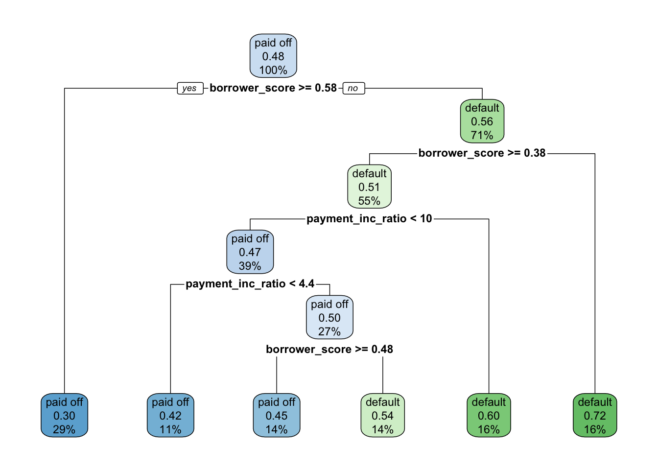

loan_tree

parsnip model object

n= 3000 

node), split, n, loss, yval, (yprob)
      * denotes terminal node

 1) root 3000 1445 paid off (0.5183333 0.4816667)  
   2) borrower_score>=0.575 878  261 paid off (0.7027335 0.2972665) *
   3) borrower_score< 0.575 2122  938 default (0.4420358 0.5579642)  
     6) borrower_score>=0.375 1639  802 default (0.4893228 0.5106772)  
      12) payment_inc_ratio< 10.42265 1157  547 paid off (0.5272256 0.4727744)  
        24) payment_inc_ratio< 4.42601 334  139 paid off (0.5838323 0.4161677) *
        25) payment_inc_ratio>=4.42601 823  408 paid off (0.5042527 0.4957473)  
          50) borrower_score>=0.475 418  190 paid off (0.5454545 0.4545455) *
          51) borrower_score< 0.475 405  187 default (0.4617284 0.5382716) *
      13) payment_inc_ratio>=10.42265 482  192 default (0.3983402 0.6016598) *
     7) borrower_score< 0.375 483  136 default (0.2815735 0.7184265) *

Bagging and the Random Forest

Random Forest

rf <- rand_forest(mode = "classification") %>%
  set_engine("ranger", seed = 123) %>%
  fit(outcome ~ borrower_score + payment_inc_ratio, data = loan3000)
rf

parsnip model object

Ranger result

Call:
 ranger::ranger(x = maybe_data_frame(x), y = y, seed = ~123, num.threads = 1,      verbose = FALSE, probability = TRUE) 

Type:                             Probability estimation 
Number of trees:                  500 
Sample size:                      3000 
Number of independent variables:  2 
Mtry:                             1 
Target node size:                 10 
Variable importance mode:         none 
Splitrule:                        gini 
OOB prediction error (Brier s.):  0.2300053 

num_trees <- c(1, seq(5, 500, 5))
oob_scores <- c()
for (trees in num_trees) {
  rf <- rand_forest(mode = "classification", trees = trees) %>%
    set_engine("ranger", seed = 123) %>%
    fit(outcome ~ borrower_score + payment_inc_ratio, data = loan3000)
  oob_scores <- c(oob_scores, (rf %>% extract_fit_engine())$prediction.error)
}
error_df <- tibble(error_rate = oob_scores, num_trees = num_trees)
ggplot(error_df, aes(x = num_trees, y = error_rate)) +
  geom_line()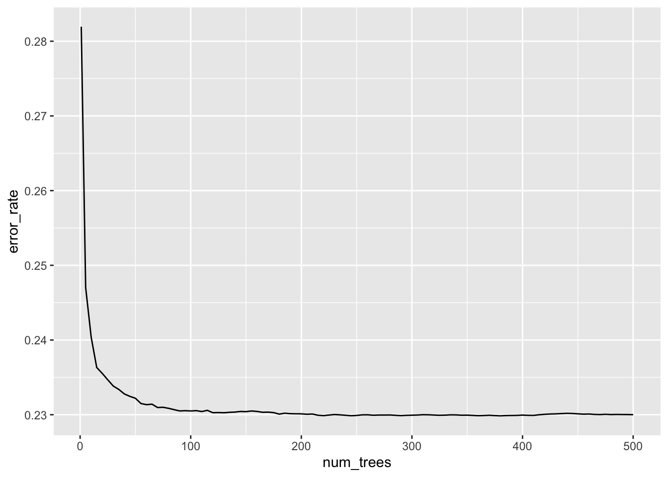

rf_df <- augment(rf, loan3000)
ggplot(data = rf_df, aes(x = borrower_score, y = payment_inc_ratio,
    shape = .pred_class, color = .pred_class, size = .pred_class)) +
  geom_jitter(alpha = 0.8, height = 0, width = 0.003) +
  scale_color_manual(values = c("paid off" = "#b8e186", "default" = "#d95f02")) +
  scale_shape_manual(values = c("paid off" = 0, "default" = 1)) +
  scale_size_manual(values = c("paid off" = 0.5, "default" = 2))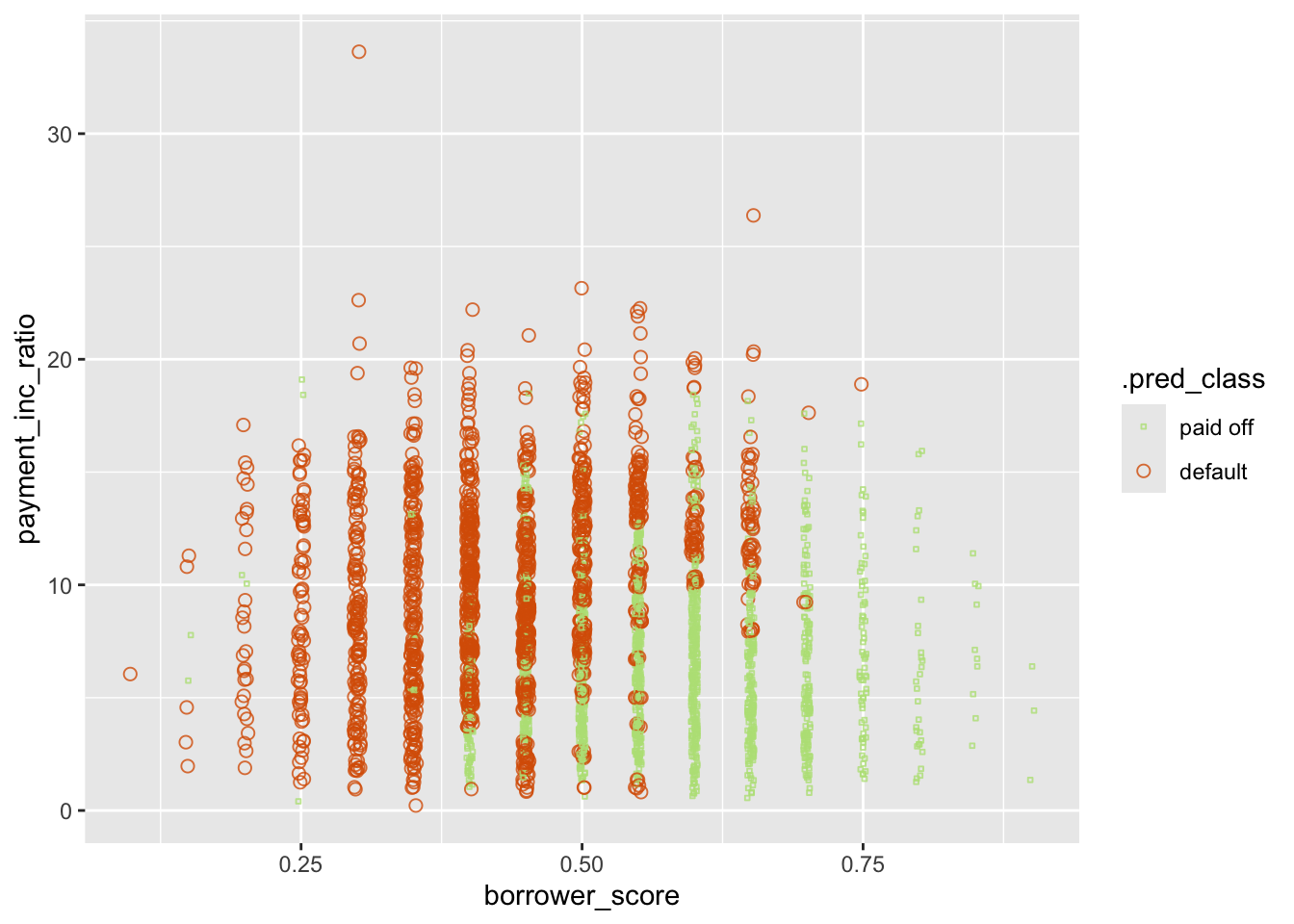

Variable Importance

rf_all <- rand_forest(mode = "classification") %>%
  set_engine("ranger", seed = 123, importance = "impurity") %>%
  fit(outcome ~ ., data = loan_data)
rf_all

parsnip model object

Ranger result

Call:
 ranger::ranger(x = maybe_data_frame(x), y = y, seed = ~123, importance = ~"impurity",      num.threads = 1, verbose = FALSE, probability = TRUE) 

Type:                             Probability estimation 
Number of trees:                  500 
Sample size:                      45342 
Number of independent variables:  18 
Mtry:                             4 
Target node size:                 10 
Variable importance mode:         impurity 
Splitrule:                        gini 
OOB prediction error (Brier s.):  0.2123043 

rf_permutation <- rand_forest(mode = "classification") %>%
  set_engine("ranger", seed = 123, importance = "permutation") %>%
  fit(outcome ~ ., data = loan_data)

varimp_gini <- importance(rf_all %>% extract_fit_engine())
varimp_perm <- importance(rf_permutation %>% extract_fit_engine())
df <- tibble(
  predictor = names(varimp_gini),
  impurity = varimp_gini,
  permutation = varimp_perm
)
g1 <- ggplot(df, aes(x = permutation, y = reorder(predictor, permutation))) +
  geom_point() +
  labs(y = "Importance", title = "Accuracy Decrease")
g2 <- ggplot(df, aes(x = impurity, y = reorder(predictor, permutation))) +
  geom_point() +
  labs(y = "Importance", title = "Gini Decrease")
(g1 + theme_bw()) / (g2 + theme_bw())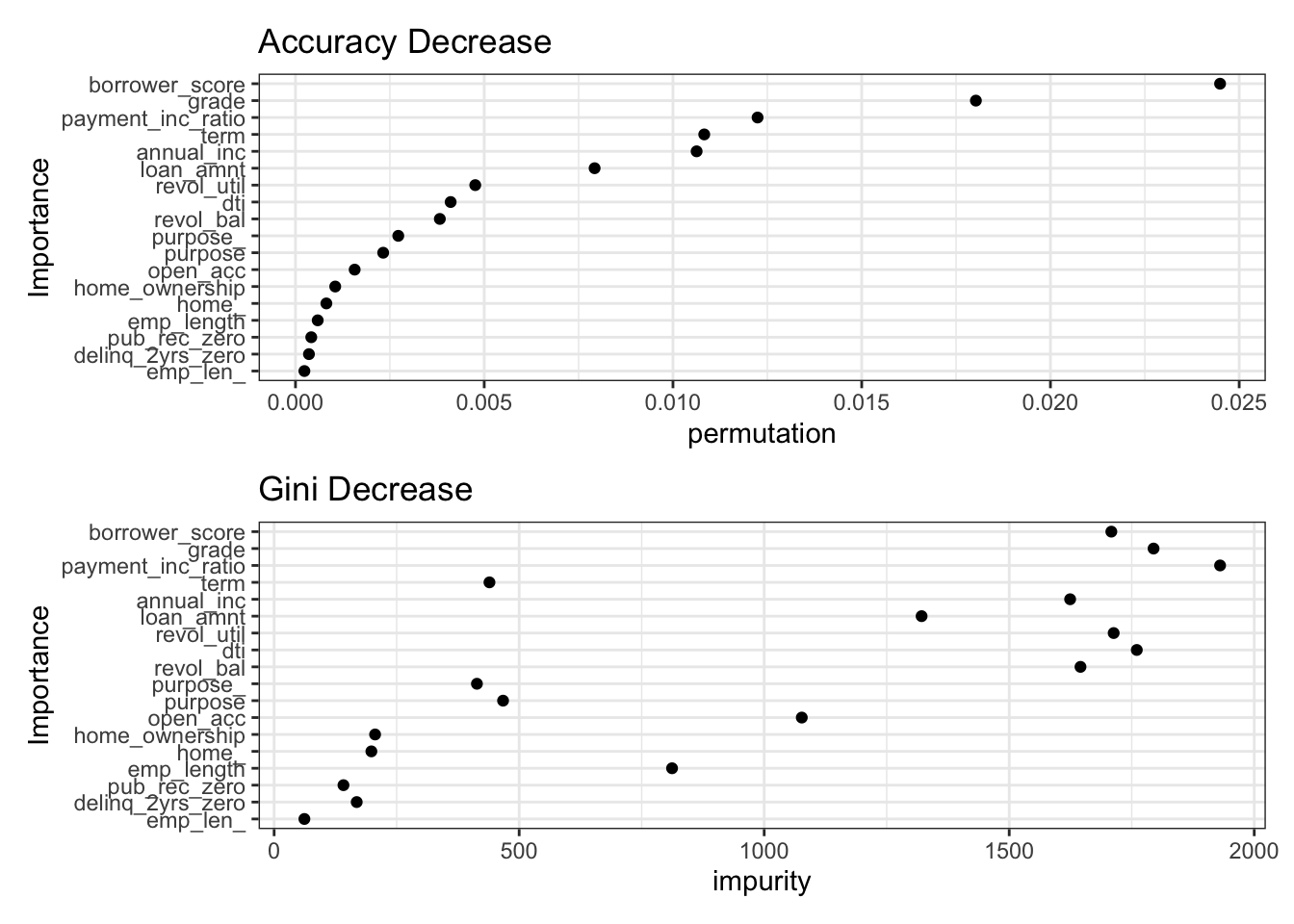

Boosting

XGBoost

xgb <- boost_tree(mode = "classification",
  trees = 100, learn_rate = 0.1, sample_size = 0.63) %>%
  fit(outcome ~ borrower_score + payment_inc_ratio, data = loan3000)

xgb_df <- augment(xgb, loan3000)
ggplot(data = xgb_df, aes(x = borrower_score, y = payment_inc_ratio,
    color = .pred_class, shape = .pred_class, size = .pred_class)) +
  geom_jitter(alpha = 0.8, height = 0, width = 0.003) +
  scale_color_manual(values = c("paid off" = "#b8e186", "default" = "#d95f02")) +
  scale_shape_manual(values = c("paid off" = 0, "default" = 1)) +
  scale_size_manual(values = c("paid off" = 0.5, "default" = 2))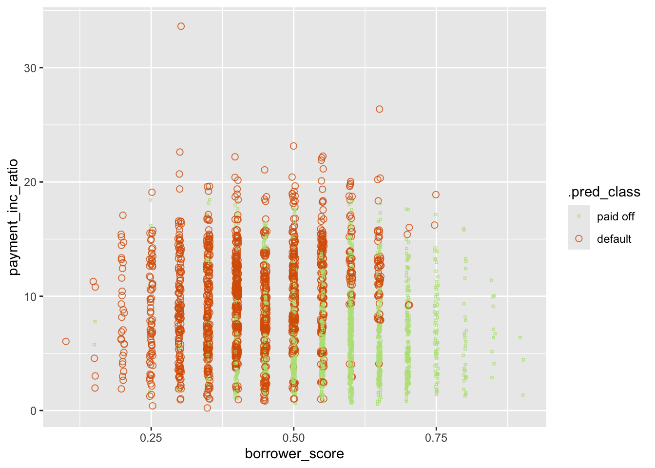

Regularization: Avoiding Overfitting

set.seed(400820)
loan_split <- initial_split(loan_data, prop = 0.75)
train_data <- training(loan_split)
test_data <- testing(loan_split)
train_x <- data.matrix(train_data %>% select(-outcome))
train_y <- factor(train_data$outcome, levels = c("paid off", "default"))
test_x <- data.matrix(test_data %>% select(-outcome))
test_y <- factor(test_data$outcome, levels = c("paid off", "default"))

xgb_default <- xgboost(x = train_x, y = train_y,
  objective = "binary:logistic", nrounds = 250, verbosity = 1,
  eval_metric = "error")

[1] train-error:0.336646 
[2] train-error:0.329677 
[3] train-error:0.326031 
[4] train-error:0.321355 
[5] train-error:0.320032 
[6] train-error:0.317356 
[7] train-error:0.315915 
[8] train-error:0.313739 
[9] train-error:0.312445 
[10]    train-error:0.311386 
[11]    train-error:0.308740 
[12]    train-error:0.306769 
[13]    train-error:0.303946 
[14]    train-error:0.302711 
[15]    train-error:0.299712 
[16]    train-error:0.298653 
[17]    train-error:0.297065 
[18]    train-error:0.296859 
[19]    train-error:0.294183 
[20]    train-error:0.293419 
[21]    train-error:0.292801 
[22]    train-error:0.290508 
[23]    train-error:0.290213 
[24]    train-error:0.288390 
[25]    train-error:0.288008 
[26]    train-error:0.287067 
[27]    train-error:0.284656 
[28]    train-error:0.283450 
[29]    train-error:0.281597 
[30]    train-error:0.280421 
[31]    train-error:0.279627 
[32]    train-error:0.278304 
[33]    train-error:0.275745 
[34]    train-error:0.274540 
[35]    train-error:0.274246 
[36]    train-error:0.273716 
[37]    train-error:0.273099 
[38]    train-error:0.271599 
[39]    train-error:0.268953 
[40]    train-error:0.267659 
[41]    train-error:0.265659 
[42]    train-error:0.264336 
[43]    train-error:0.262689 
[44]    train-error:0.260983 
[45]    train-error:0.259013 
[46]    train-error:0.257925 
[47]    train-error:0.255955 
[48]    train-error:0.255014 
[49]    train-error:0.254573 
[50]    train-error:0.253338 
[51]    train-error:0.252161 
[52]    train-error:0.251220 
[53]    train-error:0.249574 
[54]    train-error:0.249044 
[55]    train-error:0.248133 
[56]    train-error:0.246604 
[57]    train-error:0.246162 
[58]    train-error:0.245398 
[59]    train-error:0.245339 
[60]    train-error:0.243516 
[61]    train-error:0.242751 
[62]    train-error:0.241252 
[63]    train-error:0.240752 
[64]    train-error:0.239752 
[65]    train-error:0.238193 
[66]    train-error:0.237282 
[67]    train-error:0.236223 
[68]    train-error:0.234812 
[69]    train-error:0.233518 
[70]    train-error:0.232606 
[71]    train-error:0.232077 
[72]    train-error:0.230753 
[73]    train-error:0.230048 
[74]    train-error:0.228607 
[75]    train-error:0.227989 
[76]    train-error:0.227372 
[77]    train-error:0.225695 
[78]    train-error:0.224813 
[79]    train-error:0.224519 
[80]    train-error:0.223519 
[81]    train-error:0.221461 
[82]    train-error:0.220814 
[83]    train-error:0.220373 
[84]    train-error:0.218608 
[85]    train-error:0.218138 
[86]    train-error:0.217932 
[87]    train-error:0.217315 
[88]    train-error:0.216991 
[89]    train-error:0.216050 
[90]    train-error:0.215344 
[91]    train-error:0.214462 
[92]    train-error:0.213286 
[93]    train-error:0.211580 
[94]    train-error:0.211492 
[95]    train-error:0.210610 
[96]    train-error:0.210198 
[97]    train-error:0.209463 
[98]    train-error:0.209198 
[99]    train-error:0.208199 
[100]   train-error:0.207434 
[101]   train-error:0.206581 
[102]   train-error:0.205346 
[103]   train-error:0.204905 
[104]   train-error:0.204317 
[105]   train-error:0.203052 
[106]   train-error:0.202053 
[107]   train-error:0.200729 
[108]   train-error:0.199406 
[109]   train-error:0.198553 
[110]   train-error:0.198524 
[111]   train-error:0.198024 
[112]   train-error:0.197642 
[113]   train-error:0.196877 
[114]   train-error:0.195583 
[115]   train-error:0.194848 
[116]   train-error:0.194083 
[117]   train-error:0.192260 
[118]   train-error:0.191025 
[119]   train-error:0.190584 
[120]   train-error:0.190114 
[121]   train-error:0.188761 
[122]   train-error:0.188555 
[123]   train-error:0.188408 
[124]   train-error:0.187673 
[125]   train-error:0.186320 
[126]   train-error:0.185732 
[127]   train-error:0.185644 
[128]   train-error:0.185203 
[129]   train-error:0.183821 
[130]   train-error:0.183291 
[131]   train-error:0.182585 
[132]   train-error:0.181644 
[133]   train-error:0.180645 
[134]   train-error:0.179792 
[135]   train-error:0.179086 
[136]   train-error:0.178027 
[137]   train-error:0.177116 
[138]   train-error:0.177116 
[139]   train-error:0.176263 
[140]   train-error:0.176087 
[141]   train-error:0.175234 
[142]   train-error:0.174999 
[143]   train-error:0.174263 
[144]   train-error:0.173205 
[145]   train-error:0.172470 
[146]   train-error:0.171529 
[147]   train-error:0.170352 
[148]   train-error:0.169794 
[149]   train-error:0.169235 
[150]   train-error:0.168676 
[151]   train-error:0.168235 
[152]   train-error:0.167529 
[153]   train-error:0.166471 
[154]   train-error:0.165853 
[155]   train-error:0.165030 
[156]   train-error:0.164442 
[157]   train-error:0.163559 
[158]   train-error:0.162883 
[159]   train-error:0.162677 
[160]   train-error:0.162148 
[161]   train-error:0.161883 
[162]   train-error:0.161560 
[163]   train-error:0.159913 
[164]   train-error:0.158707 
[165]   train-error:0.157560 
[166]   train-error:0.157031 
[167]   train-error:0.157119 
[168]   train-error:0.156325 
[169]   train-error:0.155737 
[170]   train-error:0.154914 
[171]   train-error:0.154296 
[172]   train-error:0.153649 
[173]   train-error:0.153061 
[174]   train-error:0.152120 
[175]   train-error:0.151414 
[176]   train-error:0.150944 
[177]   train-error:0.150179 
[178]   train-error:0.149856 
[179]   train-error:0.149503 
[180]   train-error:0.149180 
[181]   train-error:0.147327 
[182]   train-error:0.146592 
[183]   train-error:0.145974 
[184]   train-error:0.145004 
[185]   train-error:0.144416 
[186]   train-error:0.144210 
[187]   train-error:0.143622 
[188]   train-error:0.143151 
[189]   train-error:0.143239 
[190]   train-error:0.142122 
[191]   train-error:0.141269 
[192]   train-error:0.140710 
[193]   train-error:0.139740 
[194]   train-error:0.139828 
[195]   train-error:0.139093 
[196]   train-error:0.138299 
[197]   train-error:0.137093 
[198]   train-error:0.137182 
[199]   train-error:0.137123 
[200]   train-error:0.137005 
[201]   train-error:0.136799 
[202]   train-error:0.135947 
[203]   train-error:0.135270 
[204]   train-error:0.133947 
[205]   train-error:0.133241 
[206]   train-error:0.132859 
[207]   train-error:0.131477 
[208]   train-error:0.130095 
[209]   train-error:0.129948 
[210]   train-error:0.129507 
[211]   train-error:0.129007 
[212]   train-error:0.128713 
[213]   train-error:0.128213 
[214]   train-error:0.127713 
[215]   train-error:0.127036 
[216]   train-error:0.126448 
[217]   train-error:0.126272 
[218]   train-error:0.125948 
[219]   train-error:0.125360 
[220]   train-error:0.125096 
[221]   train-error:0.124302 
[222]   train-error:0.123596 
[223]   train-error:0.123449 
[224]   train-error:0.122919 
[225]   train-error:0.122008 
[226]   train-error:0.121420 
[227]   train-error:0.120979 
[228]   train-error:0.120214 
[229]   train-error:0.119744 
[230]   train-error:0.118773 
[231]   train-error:0.118097 
[232]   train-error:0.117215 
[233]   train-error:0.117038 
[234]   train-error:0.116215 
[235]   train-error:0.115715 
[236]   train-error:0.115244 
[237]   train-error:0.114597 
[238]   train-error:0.114215 
[239]   train-error:0.113451 
[240]   train-error:0.112598 
[241]   train-error:0.112333 
[242]   train-error:0.112627 
[243]   train-error:0.112392 
[244]   train-error:0.112098 
[245]   train-error:0.111304 
[246]   train-error:0.110657 
[247]   train-error:0.110363 
[248]   train-error:0.110039 
[249]   train-error:0.109392 
[250]   train-error:0.108775 

pred_default <- predict(xgb_default, test_x)
error_default <- abs((as.numeric(test_y) - 1) - pred_default) > 0.5
attributes(xgb_default)$evaluation_log[250, ]

    iter train_error
   <num>       <num>
1:   250   0.1087749

mean(error_default)

[1] 0.3591214

xgb_penalty <- xgboost(x = train_x, y = train_y,
  learning_rate = 0.1, subsample = 0.63, reg_lambda = 1000,
  objective = "binary:logistic", nrounds = 250, verbosity = 1,
  eval_metric = "error")

[1] train-error:0.363730 
[2] train-error:0.344116 
[3] train-error:0.342969 
[4] train-error:0.340116 
[5] train-error:0.338646 
[6] train-error:0.334882 
[7] train-error:0.336411 
[8] train-error:0.336588 
[9] train-error:0.336911 
[10]    train-error:0.336999 
[11]    train-error:0.335588 
[12]    train-error:0.337176 
[13]    train-error:0.335794 
[14]    train-error:0.334529 
[15]    train-error:0.335676 
[16]    train-error:0.334147 
[17]    train-error:0.334323 
[18]    train-error:0.333970 
[19]    train-error:0.334323 
[20]    train-error:0.334706 
[21]    train-error:0.334118 
[22]    train-error:0.333765 
[23]    train-error:0.333118 
[24]    train-error:0.332765 
[25]    train-error:0.331294 
[26]    train-error:0.331294 
[27]    train-error:0.331353 
[28]    train-error:0.331324 
[29]    train-error:0.331236 
[30]    train-error:0.330559 
[31]    train-error:0.330530 
[32]    train-error:0.329854 
[33]    train-error:0.328971 
[34]    train-error:0.329060 
[35]    train-error:0.328530 
[36]    train-error:0.329089 
[37]    train-error:0.328471 
[38]    train-error:0.328413 
[39]    train-error:0.328295 
[40]    train-error:0.328354 
[41]    train-error:0.328030 
[42]    train-error:0.327677 
[43]    train-error:0.327530 
[44]    train-error:0.326913 
[45]    train-error:0.327178 
[46]    train-error:0.327295 
[47]    train-error:0.327295 
[48]    train-error:0.326678 
[49]    train-error:0.326413 
[50]    train-error:0.326119 
[51]    train-error:0.326678 
[52]    train-error:0.326913 
[53]    train-error:0.326442 
[54]    train-error:0.326119 
[55]    train-error:0.325795 
[56]    train-error:0.326060 
[57]    train-error:0.325884 
[58]    train-error:0.325472 
[59]    train-error:0.325296 
[60]    train-error:0.325119 
[61]    train-error:0.324943 
[62]    train-error:0.324796 
[63]    train-error:0.324355 
[64]    train-error:0.324619 
[65]    train-error:0.324472 
[66]    train-error:0.324119 
[67]    train-error:0.324443 
[68]    train-error:0.324266 
[69]    train-error:0.324119 
[70]    train-error:0.323708 
[71]    train-error:0.323913 
[72]    train-error:0.323472 
[73]    train-error:0.323855 
[74]    train-error:0.323825 
[75]    train-error:0.323855 
[76]    train-error:0.324237 
[77]    train-error:0.324031 
[78]    train-error:0.323796 
[79]    train-error:0.323590 
[80]    train-error:0.323590 
[81]    train-error:0.323561 
[82]    train-error:0.323296 
[83]    train-error:0.322855 
[84]    train-error:0.323002 
[85]    train-error:0.322825 
[86]    train-error:0.322649 
[87]    train-error:0.322473 
[88]    train-error:0.322267 
[89]    train-error:0.322561 
[90]    train-error:0.322502 
[91]    train-error:0.322296 
[92]    train-error:0.321884 
[93]    train-error:0.321826 
[94]    train-error:0.321737 
[95]    train-error:0.321826 
[96]    train-error:0.321855 
[97]    train-error:0.321679 
[98]    train-error:0.321767 
[99]    train-error:0.321414 
[100]   train-error:0.321502 
[101]   train-error:0.321561 
[102]   train-error:0.321237 
[103]   train-error:0.321326 
[104]   train-error:0.321090 
[105]   train-error:0.321032 
[106]   train-error:0.320532 
[107]   train-error:0.320826 
[108]   train-error:0.321002 
[109]   train-error:0.321179 
[110]   train-error:0.320796 
[111]   train-error:0.320826 
[112]   train-error:0.320943 
[113]   train-error:0.320796 
[114]   train-error:0.320590 
[115]   train-error:0.320738 
[116]   train-error:0.320826 
[117]   train-error:0.320355 
[118]   train-error:0.320414 
[119]   train-error:0.320649 
[120]   train-error:0.320267 
[121]   train-error:0.320385 
[122]   train-error:0.320502 
[123]   train-error:0.320473 
[124]   train-error:0.320208 
[125]   train-error:0.320355 
[126]   train-error:0.320149 
[127]   train-error:0.319944 
[128]   train-error:0.319944 
[129]   train-error:0.319973 
[130]   train-error:0.319738 
[131]   train-error:0.319855 
[132]   train-error:0.319738 
[133]   train-error:0.319649 
[134]   train-error:0.319708 
[135]   train-error:0.319708 
[136]   train-error:0.319473 
[137]   train-error:0.319208 
[138]   train-error:0.319179 
[139]   train-error:0.319120 
[140]   train-error:0.319032 
[141]   train-error:0.318797 
[142]   train-error:0.318708 
[143]   train-error:0.318738 
[144]   train-error:0.319032 
[145]   train-error:0.318620 
[146]   train-error:0.318503 
[147]   train-error:0.318238 
[148]   train-error:0.318091 
[149]   train-error:0.317973 
[150]   train-error:0.318062 
[151]   train-error:0.318297 
[152]   train-error:0.318150 
[153]   train-error:0.318297 
[154]   train-error:0.317856 
[155]   train-error:0.318091 
[156]   train-error:0.317709 
[157]   train-error:0.317620 
[158]   train-error:0.317591 
[159]   train-error:0.317738 
[160]   train-error:0.317503 
[161]   train-error:0.317562 
[162]   train-error:0.317268 
[163]   train-error:0.317297 
[164]   train-error:0.317003 
[165]   train-error:0.317003 
[166]   train-error:0.317121 
[167]   train-error:0.316885 
[168]   train-error:0.316621 
[169]   train-error:0.316621 
[170]   train-error:0.316709 
[171]   train-error:0.316474 
[172]   train-error:0.316268 
[173]   train-error:0.316385 
[174]   train-error:0.316062 
[175]   train-error:0.316474 
[176]   train-error:0.316444 
[177]   train-error:0.316179 
[178]   train-error:0.315944 
[179]   train-error:0.316091 
[180]   train-error:0.316032 
[181]   train-error:0.315768 
[182]   train-error:0.315915 
[183]   train-error:0.315974 
[184]   train-error:0.316268 
[185]   train-error:0.315621 
[186]   train-error:0.315768 
[187]   train-error:0.315797 
[188]   train-error:0.315650 
[189]   train-error:0.315474 
[190]   train-error:0.315533 
[191]   train-error:0.315297 
[192]   train-error:0.315268 
[193]   train-error:0.315033 
[194]   train-error:0.315003 
[195]   train-error:0.315003 
[196]   train-error:0.315268 
[197]   train-error:0.314915 
[198]   train-error:0.314386 
[199]   train-error:0.314533 
[200]   train-error:0.314092 
[201]   train-error:0.314121 
[202]   train-error:0.314209 
[203]   train-error:0.314121 
[204]   train-error:0.314209 
[205]   train-error:0.314033 
[206]   train-error:0.314003 
[207]   train-error:0.313886 
[208]   train-error:0.313886 
[209]   train-error:0.313768 
[210]   train-error:0.313886 
[211]   train-error:0.313798 
[212]   train-error:0.313915 
[213]   train-error:0.313356 
[214]   train-error:0.313209 
[215]   train-error:0.313592 
[216]   train-error:0.313151 
[217]   train-error:0.313445 
[218]   train-error:0.313356 
[219]   train-error:0.313474 
[220]   train-error:0.313474 
[221]   train-error:0.313356 
[222]   train-error:0.313151 
[223]   train-error:0.313062 
[224]   train-error:0.312680 
[225]   train-error:0.312886 
[226]   train-error:0.313180 
[227]   train-error:0.312915 
[228]   train-error:0.312474 
[229]   train-error:0.312504 
[230]   train-error:0.312415 
[231]   train-error:0.312474 
[232]   train-error:0.312092 
[233]   train-error:0.311592 
[234]   train-error:0.311827 
[235]   train-error:0.311739 
[236]   train-error:0.311769 
[237]   train-error:0.311798 
[238]   train-error:0.311474 
[239]   train-error:0.311621 
[240]   train-error:0.311621 
[241]   train-error:0.311416 
[242]   train-error:0.310916 
[243]   train-error:0.311092 
[244]   train-error:0.311092 
[245]   train-error:0.310769 
[246]   train-error:0.310975 
[247]   train-error:0.310504 
[248]   train-error:0.310680 
[249]   train-error:0.310181 
[250]   train-error:0.310210 

pred_penalty <- predict(xgb_penalty, test_x)
error_penalty <- abs((as.numeric(test_y) - 1) - pred_penalty) > 0.5
attributes(xgb_penalty)$evaluation_log[250, ]

    iter train_error
   <num>       <num>
1:   250     0.31021

mean(error_penalty)

[1] 0.3300988

error_default <- rep(0, 249)
error_penalty <- rep(0, 249)
for (ntree_limit in 1:249) {
  iteration_range <- c(1, ntree_limit + 1)
  pred_def <- predict(xgb_default, test_x, iteration_range = iteration_range)
  error_default[ntree_limit] <- mean(abs(as.numeric(test_y)-1-pred_def) >= 0.5)
  pred_pen <- predict(xgb_penalty, test_x, iteration_range = iteration_range)
  error_penalty[ntree_limit] <- mean(abs(as.numeric(test_y)-1-pred_pen) >= 0.5)
}

errors <- bind_rows(
  tibble(Iterations = 1:250, Dataset = "train", Penalty = "no",
    Error = attributes(xgb_default)$evaluation_log$train_error),
  tibble(Iterations = 1:249, Dataset = "test", Penalty = "no",
    Error = error_default),
  tibble(Iterations = 1:250, Dataset = "train", Penalty = "yes",
    Error = attributes(xgb_penalty)$evaluation_log$train_error),
  tibble(Iterations = 1:249, Dataset = "test", Penalty = "yes",
    Error = error_penalty),
)
ggplot(errors, aes(x = Iterations, y = Error, color = Penalty,
    linetype = Dataset)) +
  geom_line() +
  scale_color_manual(values = c("red", "black"))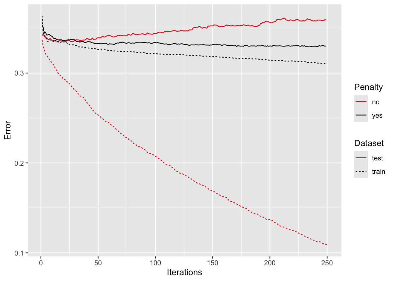

last_plot()  +
  theme_bw() +
  annotate("text", 165, 0.2, label="Default / Training set") +
  annotate("text", 150, 0.3, label="Penalty / Training set") +
  annotate("text", 220, 0.34, label="Penalty / Test set") +
  annotate("text", 75, 0.36, label="Default / Test set") +
  theme(legend.position = "none")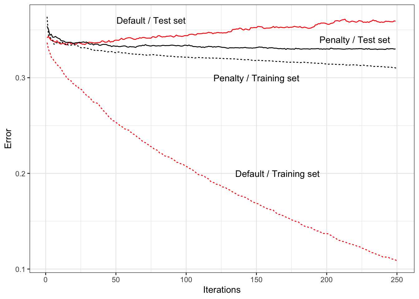

Hyperparameters and Cross-Validation

set.seed(1234)
resamples <- vfold_cv(loan_data, v = 5)
grid <- crossing(
  tree_depth = c(3, 6, 12),
  learn_rate = c(0.1, 0.5, 0.9),
)

plan(multisession, workers = parallel::detectCores(logical = FALSE))

rec <- recipe(outcome ~ ., data = loan_data) %>%
  step_dummy(all_nominal_predictors())
model <- boost_tree(mode = "classification",
  tree_depth = tune(), learn_rate = tune())

wf <- workflow() %>%
  add_model(model) %>%
  add_recipe(rec)

model_cv <- tune_grid(wf, resamples, grid = grid)

collect_metrics(model_cv) %>%
  filter(.metric == "accuracy") %>%
  mutate(error_rate = round(100 * (1 - mean), 2)) %>%
  select(c(tree_depth, learn_rate, error_rate)) %>%
  arrange(error_rate)

# A tibble: 9 × 3
  tree_depth learn_rate error_rate
       <dbl>      <dbl>      <dbl>
1          3        0.5       33.3
2          3        0.9       33.5
3          6        0.1       33.5
4          6        0.5       33.8
5          3        0.1       34.2
6         12        0.1       34.7
7          6        0.9       34.9
8         12        0.5       36.4
9         12        0.9       38.8

Supplementary Material

Figure 6-2. KNN prediction of loan default using two variables: debt-to-income ratio and loan-payment-to-income ratio

train_data <- loan200 %>%
  dplyr::slice(-1)
newloan <- loan200 %>%
  dplyr::slice(1) %>%
  select(payment_inc_ratio, dti)

# The knn function from the class package gives us access to a list of the nearest
# neighbors and their distances via attributes "nn.index" and "nn.dist"
knn_pred <- knn(train = train_data[c("payment_inc_ratio", "dti")], test = newloan,
  cl = train_data$outcome, k = 20)

nearest_points <- loan200[c(attr(knn_pred, "nn.index") + 1), ]
nearest_points

# A tibble: 20 × 3
   outcome  payment_inc_ratio   dti
   <fct>                <dbl> <dbl>
 1 default               8.66  22.2
 2 default               9.06  21.6
 3 paid off              9.45  23.3
 4 default               8.71  24.1
 5 default               9.43  24.2
 6 default               8.03  20.9
 7 default               6.92  22.5
 8 paid off              9.64  20.2
 9 paid off              7.70  24.6
10 paid off             11.5   21.4
11 paid off              8.65  19.8
12 paid off             11.9   22.5
13 paid off              9.52  19.7
14 paid off              7.90  19.7
15 paid off             10.2   25.5
16 default               5.82  22  
17 default              12.4   22.2
18 paid off              5.62  22.4
19 paid off              8.16  19.1
20 default              10.0   19.1

dist <- attr(knn_pred, "nn.dist")

circle_coordinates <- function(center = c(0, 0), r = 1, npoints = 100) {
  tt <- seq(0, 2 * pi, length.out = npoints - 1)
  xx <- center[1] + r * cos(tt)
  yy <- center[2] + r * sin(tt)
  return(data.frame(x = c(xx, xx[1]), y = c(yy, yy[1])))
}

circle_df <- circle_coordinates(center = unlist(newloan), r = max(dist),
  npoints = 201)

# set first entry as target - requires adding additional level to factor
levels(loan200$outcome) <- c(levels(loan200$outcome), "newloan")
loan200[1, "outcome"] <- "newloan"
head(loan200)

# A tibble: 6 × 3
  outcome  payment_inc_ratio   dti
  <fct>                <dbl> <dbl>
1 newloan               9    22.5 
2 default               5.47 21.3 
3 paid off              6.90  8.97
4 paid off             11.1   1.83
5 default               3.72 10.8 
6 paid off              1.90 11.3 

levels(nearest_points$outcome)

[1] "paid off" "default" 

graph <- ggplot(data = loan200, aes(x = payment_inc_ratio, y = dti, color = outcome)) +
  geom_point(aes(shape = outcome), size = 2, alpha = 0.4) +
  geom_point(data = nearest_points, aes(shape = outcome), size = 2) +
  geom_point(data = loan200[1, ], aes(shape = outcome), size = 2) +
  scale_shape_manual(values = c(15, 16, 4)) +
  scale_color_manual(values = c("paid off" = "#1b9e77", "default" = "#d95f02", "newloan" = "black")) +
  geom_path(data = circle_df, aes(x = x, y = y), color = "black") +
  coord_cartesian(xlim = c(3, 15), ylim = c(17, 29)) +
  theme_bw()
graph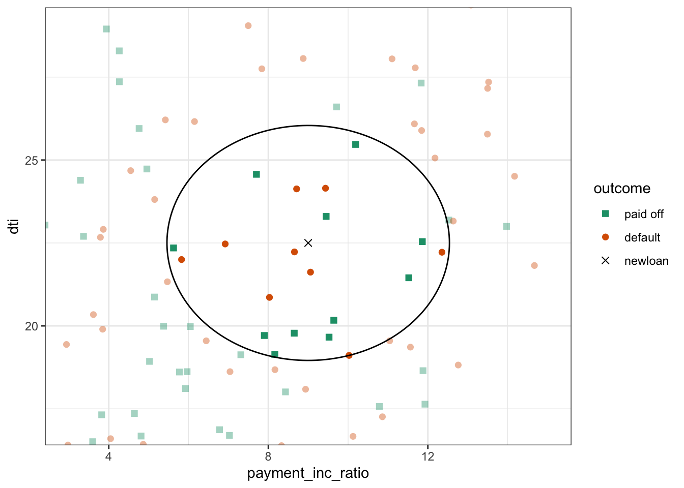

Figure 6-4. The first five rules for a simple tree model fit to the loan data

## Figure 6-4: View of partition rules
r_tree <- tibble(
  x1 = c(0.575, 0.375, 0.375, 0.375, 0.475),
  x2 = c(0.575, 0.375, 0.575, 0.575, 0.475),
  y1 = c(0, 0, 10.42, 4.426, 4.426),
  y2 = c(25, 25, 10.42, 4.426, 10.42),
  rule_number = factor(c(1, 2, 3, 4, 5)))
r_tree <- as.data.frame(r_tree)

rules <- tibble(
  x = c(0.575, 0.375, 0.4, 0.4, 0.475),
  y = c(24, 24, 10.42, 4.426, 9.42),
  rule_number = factor(c(1, 2, 3, 4, 5))
)

labs <- tibble(
  x = c(
    0.575 + (1 - 0.575) / 2,
    0.375 / 2,
    (0.375 + 0.575) / 2,
    (0.375 + 0.575) / 2,
    (0.475 + 0.575) / 2,
    (0.375 + 0.475) / 2
  ),
  y = c(
    12.5,
    12.5,
    10.42 + (25 - 10.42) / 2,
    4.426 / 2,
    4.426 + (10.42 - 4.426) / 2,
    4.426 + (10.42 - 4.426) / 2
  ),
  decision = factor(c(
    "paid off",
    "default",
    "default",
    "paid off",
    "paid off",
    "default"
  ))
)

shift <- 0.004
shift <- 0
graph <- loan3000 %>%
  #  mutate(borrower_score = ifelse(outcome == "paid off", borrower_score + shift, borrower_score - shift)) %>%
  mutate(
    borrower_score = borrower_score + rnorm(dim(loan3000)[1], sd = 2 * shift)
  ) %>%
  ggplot(aes(x = borrower_score, y = payment_inc_ratio)) +
    geom_point(aes(color = outcome, size = outcome, shape = outcome), alpha = 0.5) +
    # scale_color_manual(values = c("paid off" = "#7fbc41", "default" = "#d95f02")) +
    scale_shape_manual(values = c("paid off" = 0, "default" = 1)) +
    scale_size_manual(values = c("paid off" = 1, "default" = 1)) +
    geom_segment(data = r_tree, aes(x = x1, y = y1, xend = x2, yend = y2), linewidth = 1.5) +
    guides(color = guide_legend(override.aes = list(linewidth = 1.5)),
      linetype = guide_legend(keywidth = 3, override.aes = list(linewidth = 1))) +
    scale_x_continuous(expand = c(0, 0)) +
    scale_y_continuous(expand = c(0, 0)) +
    coord_cartesian(ylim = c(0, 25)) +
    geom_label(data = labs, aes(x = x, y = y, label = decision)) +
    geom_label(data = rules, aes(x = x, y = y, label = rule_number),
      size = 2.5, fill = "#eeeeee",
      label.r = unit(0, "lines"), label.padding = unit(0.2, "lines")) +
    guides(color = guide_legend(override.aes = list(size = 2))) +
    stat_density_2d(aes(linetype = outcome, color = outcome),  
    # variation geom = "polygon",
    # variation aes(alpha = 0.1 * ..level.., fill = outcome),
                    bins = 6)  +
    theme_bw()
graph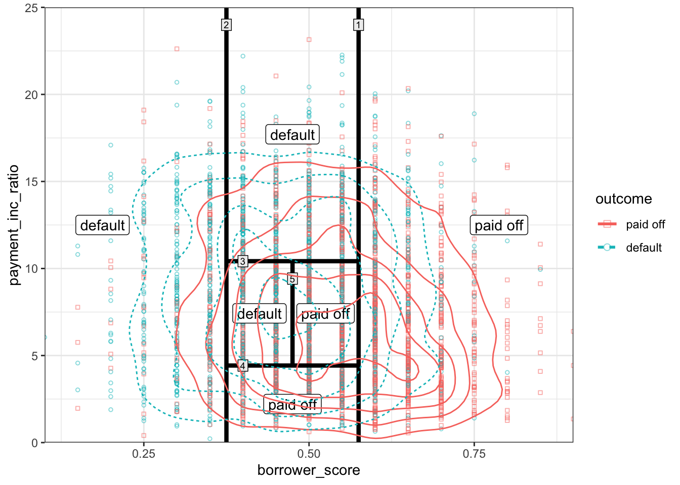

graph <- ggplot(data = loan3000, aes(x = borrower_score, y = payment_inc_ratio)) +
  geom_point(aes(color = outcome, shape = outcome, size = outcome), alpha = 0.8) +
  scale_color_manual(values = c("paid off" = "#7fbc41", "default" = "#d95f02")) +
  scale_shape_manual(values = c("paid off" = 0, "default" = 1)) +
  scale_size_manual(values = c("paid off" = 0.5, "default" = 2)) +
  geom_segment(data = r_tree, aes(x = x1, y = y1, xend = x2, yend = y2), size = 1.5) +
  guides(color = guide_legend(override.aes = list(size = 1.5)),
    linetype = guide_legend(keywidth = 3, override.aes = list(size = 1))) +
  scale_x_continuous(expand = c(0, 0)) +
  scale_y_continuous(expand = c(0, 0)) +
  coord_cartesian(ylim = c(0, 25)) +
  geom_label(data = labs, aes(x = x, y = y, label = decision)) +
  geom_label(data = rules, aes(x = x, y = y, label = rule_number),
    size = 2.5, fill = "#eeeeee",
    label.r = unit(0, "lines"), label.padding = unit(0.2, "lines")) +
  guides(color = guide_legend(override.aes = list(size = 2))) +
  theme_bw()

Warning: Using `size` aesthetic for lines was deprecated in ggplot2 3.4.0.
ℹ Please use `linewidth` instead.

graph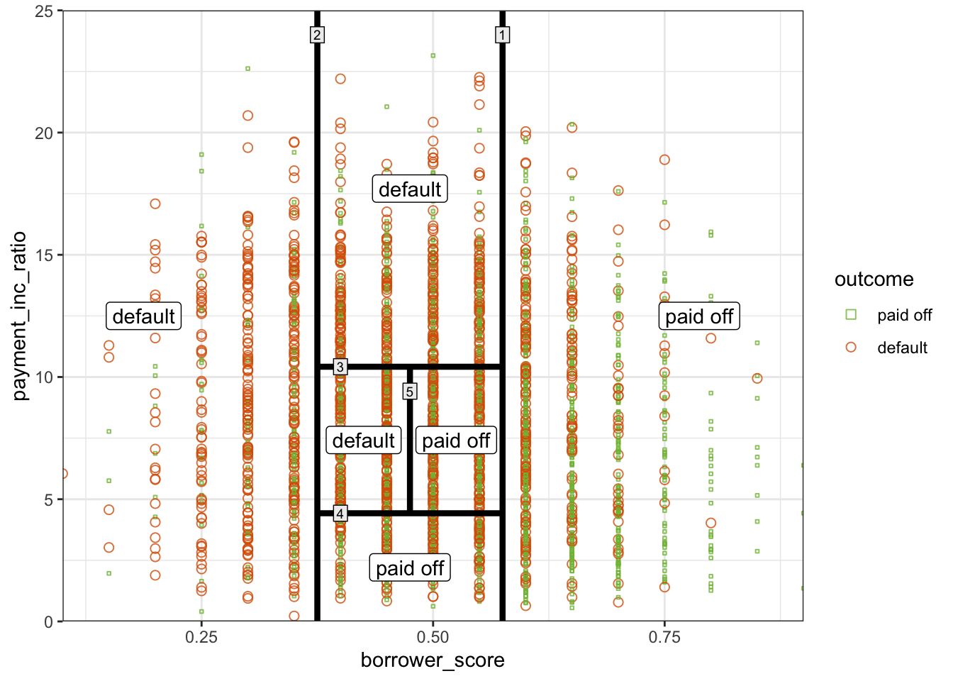

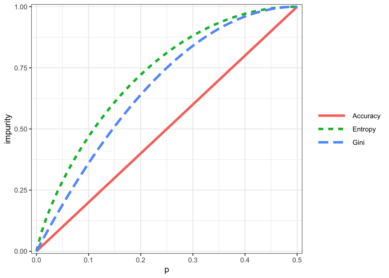
Figure 6-5. Gini impurity and entropy measures

info <- function(x) {
  info <- ifelse(x == 0, 0, -x * log2(x) - (1 - x) * log2(1 - x))
  return(info)
}

gini <- function(x) {
  return(x * (1 - x))
}

x <- 0:50 / 100
impure <- bind_rows(
  tibble(p = x, impurity = 2 * x, type = "Accuracy"),
  tibble(p = x, impurity = gini(x) / gini(0.5) * info(0.5), type = "Gini"),
  tibble(p = x, impurity = info(x), type = "Entropy")
)

graph <- ggplot(data = impure, aes(x = p, y = impurity, linetype = type, color = type)) +
  geom_line(size = 1.5) +
  guides(linetype = guide_legend(keywidth = 3, override.aes = list(size = 1))) +
  scale_x_continuous(expand = c(0, 0.01)) +
  scale_y_continuous(expand = c(0, 0.01)) +
  theme_bw() +
  theme(legend.title = element_blank())
graph