Chapter 1: Exploratory Data Analysis

library(corrplot)
library(ellmer)
library(gmodels)
library(matrixStats)
library(tidyverse)

set.seed(123)

# Location of the data files. Adjust this path if you keep the data
# files in a different directory.
DATA_DIR <- '../data'

Exploratory Data Analysis

Data Dictionaries and Catalogs

system_prompt <- "
Improve the attached data dictionary and return it in YAML format. In addition to
the description of features, provide name, description, source, and
size of the dataset.

For each feature, provide the following information:
- feature name
- readable variable name (if required)
- definition of the variable
- data type
- measurement units
- allowed values (for categorical or nominal features, but only if you are sure)
"

data_dictionary <- "
name: ebay Auctions
description: >
    The dataset eBayAuctions.csv contains information on 1972 auctions that
    transacted on eBay.com during May-June 2004.
source: Copyright 2016 Galit Shmueli and Peter Bruce
size:
    observations: 1972
    features: 8
features:
    Category: Category of the auctioned item
    currency: \"US: US dollar, GBP: English pound, EUR: Euro\"
    sellerRating: >
        a rating by eBay, as a function of the number of \"good\" and  \"bad\"
        transactions the seller had on eBay
    Duration: Number of days the auction lasted (set by seller at auction start)
    endDay: Day of week that the auction closed
    ClosePrice: Price item sold at (converted into USD)
    OpenPrice: Initial price set by the seller (converted into USD)
    Competitive?: whether the auction had a single bid (0) or more (1)
"

message <- paste(c(
  "Here is the data dictionary in YAML format:",
  data_dictionary,
  "First ten lines of the dataset in CSV format:",
  read_csv(file.path(DATA_DIR, "eBayAuctions.csv.gz"), show_col_types = FALSE) %>%
    sample_n(10) %>%
    format_delim(delim = ",", na = "")
), collapse = "\n")

chat <- chat_openai(system_prompt, model = "gpt-4o-mini")
response <- chat$chat(message)

Here’s an improved version of your data dictionary in YAML format:

```yaml
name: ebay Auctions
description: >
    The dataset eBayAuctions.csv contains information on 1972 auctions that
    were transacted on eBay.com during May-June 2004.
source: Copyright 2016 Galit Shmueli and Peter Bruce
size:
    observations: 1972
    features: 8
features:
  - feature_name: Category
    readable_variable_name: Auction Category
    definition: Category of the auctioned item
    data_type: categorical
    allowed_values: 
      - Music/Movie/Game
      - Coins/Stamps
      - Automotive
      - Health/Beauty
      - Toys/Hobbies
      - Collectibles

  - feature_name: currency
    readable_variable_name: Currency Type
    definition: Currency used for the auction prices
    data_type: categorical
    allowed_values: 
      - US
      - GBP
      - EUR

  - feature_name: sellerRating
    readable_variable_name: Seller Rating
    definition: A rating by eBay based on the number of 'good' and 'bad' 
transactions the seller had
    data_type: integer
    measurement_units: rating scale

  - feature_name: Duration
    readable_variable_name: Auction Duration
    definition: Number of days the auction lasted (set by seller at auction 
start)
    data_type: integer
    measurement_units: days

  - feature_name: endDay
    readable_variable_name: End Day of Auction
    definition: Day of the week that the auction closed
    data_type: categorical
    allowed_values:
      - Mon
      - Tue
      - Wed
      - Thu
      - Fri
      - Sat
      - Sun

  - feature_name: ClosePrice
    readable_variable_name: Closing Price
    definition: Price at which the item sold (converted into USD)
    data_type: float
    measurement_units: USD

  - feature_name: OpenPrice
    readable_variable_name: Opening Price
    definition: Initial price set by the seller (converted into USD)
    data_type: float
    measurement_units: USD

  - feature_name: Competitive
    readable_variable_name: Competitive Bidding
    definition: Indicates whether the auction had a single bid (0) or more (1)
    data_type: categorical
    allowed_values:
      - 0: Single Bid
      - 1: Multiple Bids
```

Feel free to let me know if you need any further modifications or additional 
information!

Estimates of Location

Example: Location Estimates of Population and Murder Rates

state <- read_csv(file.path(DATA_DIR, "state.csv"), show_col_types = FALSE)
population <- state[["Population"]]
mean(population)

[1] 6162876

mean(population, trim = 0.1)

[1] 4783697

median(population)

[1] 4436370

weighted.mean(state[["Murder.Rate"]], w = state[["Population"]])

[1] 4.445834

weightedMedian(state[["Murder.Rate"]], w = state[["Population"]])

[1] 4.4

Estimates of Variability

Example: Variability Estimates of State Population

sd(state[["Population"]])

[1] 6848235

IQR(state[["Population"]])

[1] 4847308

mad(state[["Population"]])

[1] 3849870

Exploring the Data Distribution

Percentiles and Boxplots

quantile(state[["Murder.Rate"]], p = c(0.05, 0.25, 0.5, 0.75, 0.95))

   5%   25%   50%   75%   95% 
1.600 2.425 4.000 5.550 6.510 

ggplot(state, aes(y = Population / 1000000)) +
  geom_boxplot(staplewidth = 0.25) +
  labs(y = "Population (millions)") +
  scale_x_discrete(labels = NULL, breaks = NULL)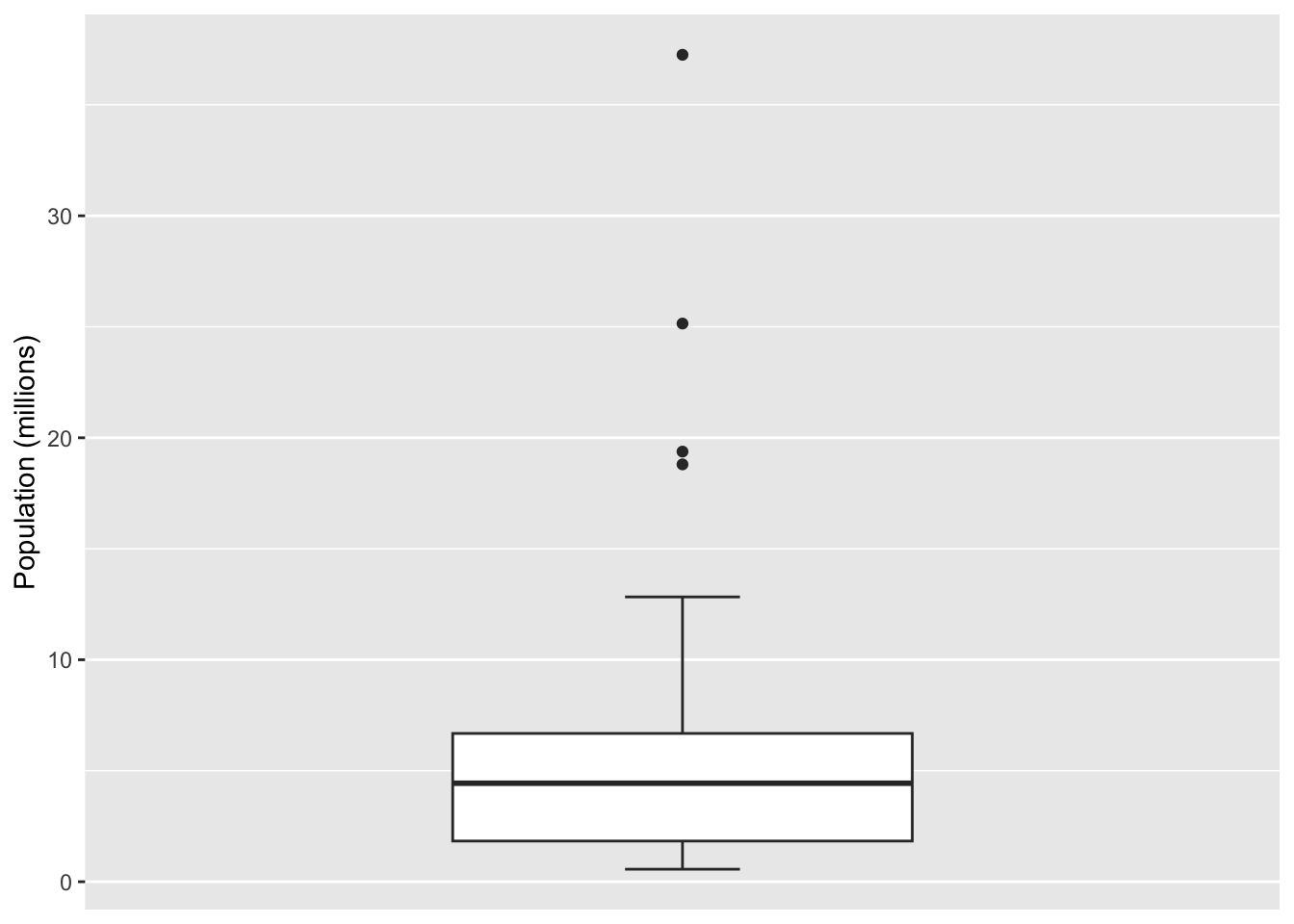

Frequency Tables and Histograms

breaks <- seq(
  from = min(state[["Population"]]),
  to = max(state[["Population"]]), length = 11)
state %>%
  mutate(BinRange = cut(Population, breaks = breaks,
      right = TRUE, include.lowest = TRUE)) %>%
  count(BinRange, .drop = FALSE)

# A tibble: 10 × 2
   BinRange                n
   <fct>               <int>
 1 [5.64e+05,4.23e+06]    24
 2 (4.23e+06,7.9e+06]     14
 3 (7.9e+06,1.16e+07]      6
 4 (1.16e+07,1.52e+07]     2
 5 (1.52e+07,1.89e+07]     1
 6 (1.89e+07,2.26e+07]     1
 7 (2.26e+07,2.62e+07]     1
 8 (2.62e+07,2.99e+07]     0
 9 (2.99e+07,3.36e+07]     0
10 (3.36e+07,3.73e+07]     1

ggplot(state, aes(x = Population)) +
  geom_histogram(breaks = breaks, fill = "grey", color = "black") +
  labs(y = "Frequency")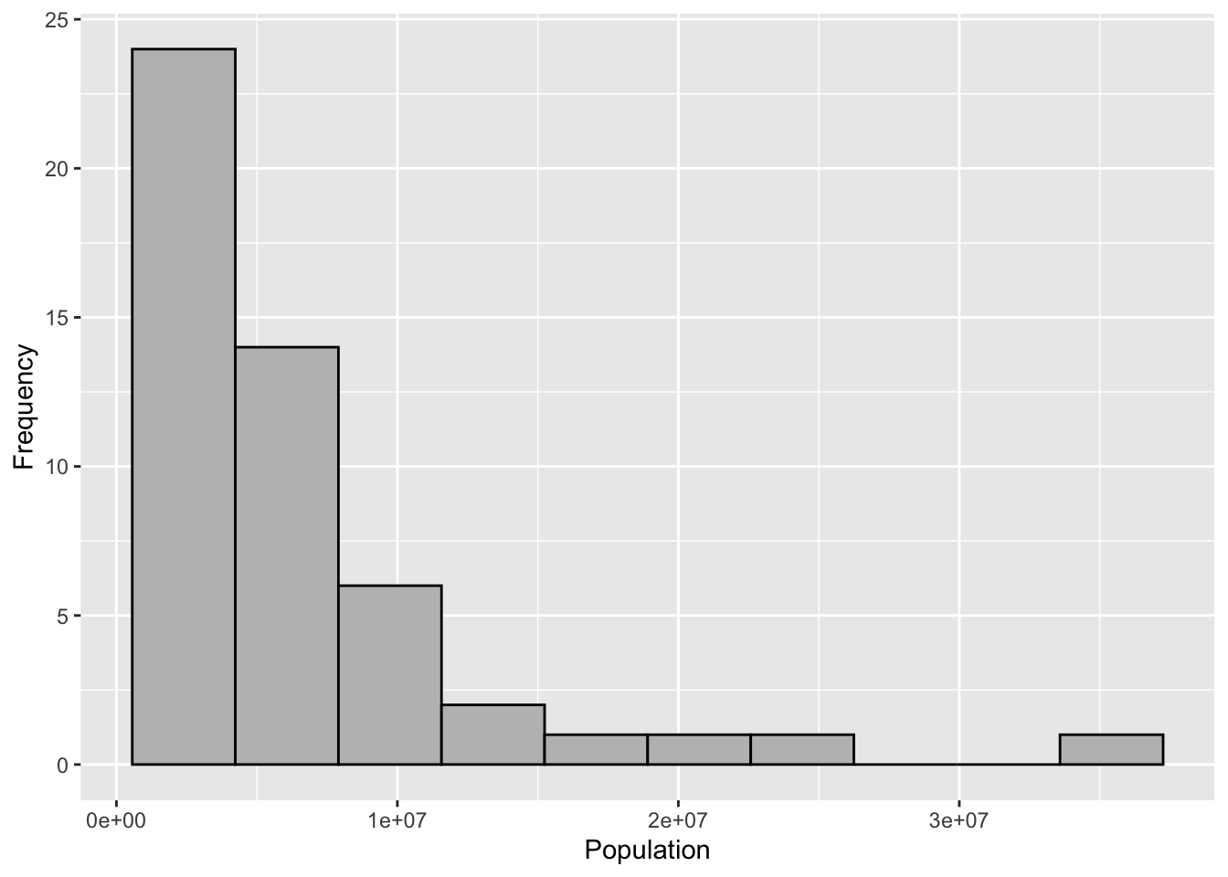

Density Plots and Estimates

ggplot(state, aes(x = Murder.Rate)) +
  geom_histogram(aes(y = after_stat(density)), bins = 12, fill = "grey",
    color = "black") +
  geom_density() +
  labs(x = "Murder Rate (per 100,000)", y = "Density")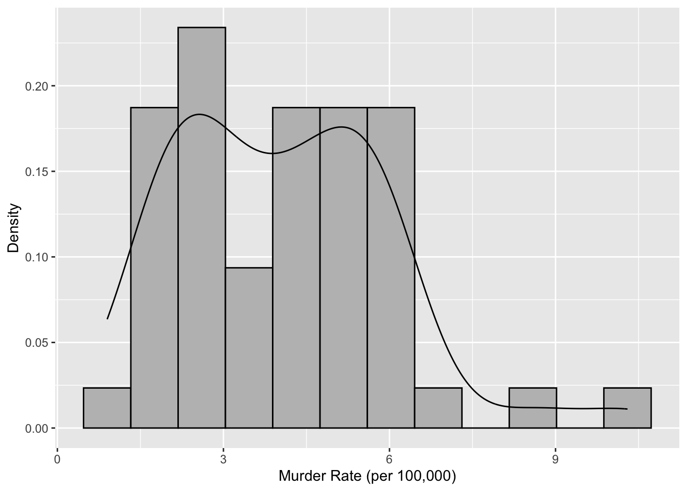

Exploring Binary and Categorical Data

dfw <- read_csv(file.path(DATA_DIR, "dfw_airline.csv"), show_col_types = FALSE) %>%
  pivot_longer(everything())
ggplot(dfw, aes(x = name, y = value)) +
  geom_col(color = "black", fill = "grey") +
  labs(x = "Cause of delay", y = "Count")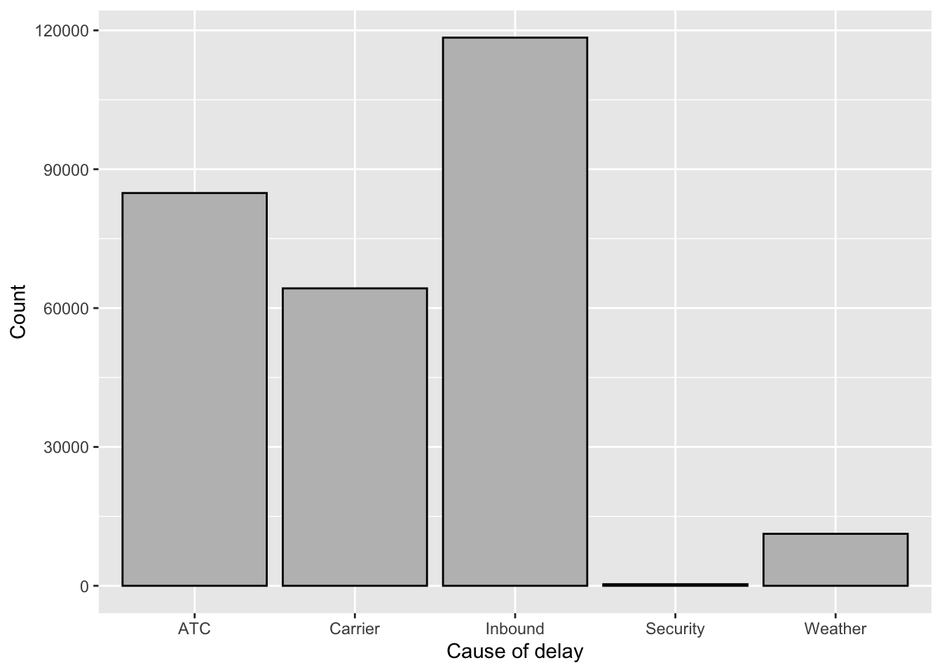

Correlation

sp500_px <- read_csv(file.path(DATA_DIR, "sp500_data.csv.gz"), show_col_types = FALSE)
sp500_sym <- read_csv(file.path(DATA_DIR, "sp500_sectors.csv"), show_col_types = FALSE)
etf_symbols <- sp500_sym %>%
  filter(sector == "etf") %>%
  pull(symbol)
etfs <- sp500_px %>%
  filter(Date > "2012-07-01") %>%
  select(all_of(etf_symbols))
corrplot(cor(etfs), method = "ellipse")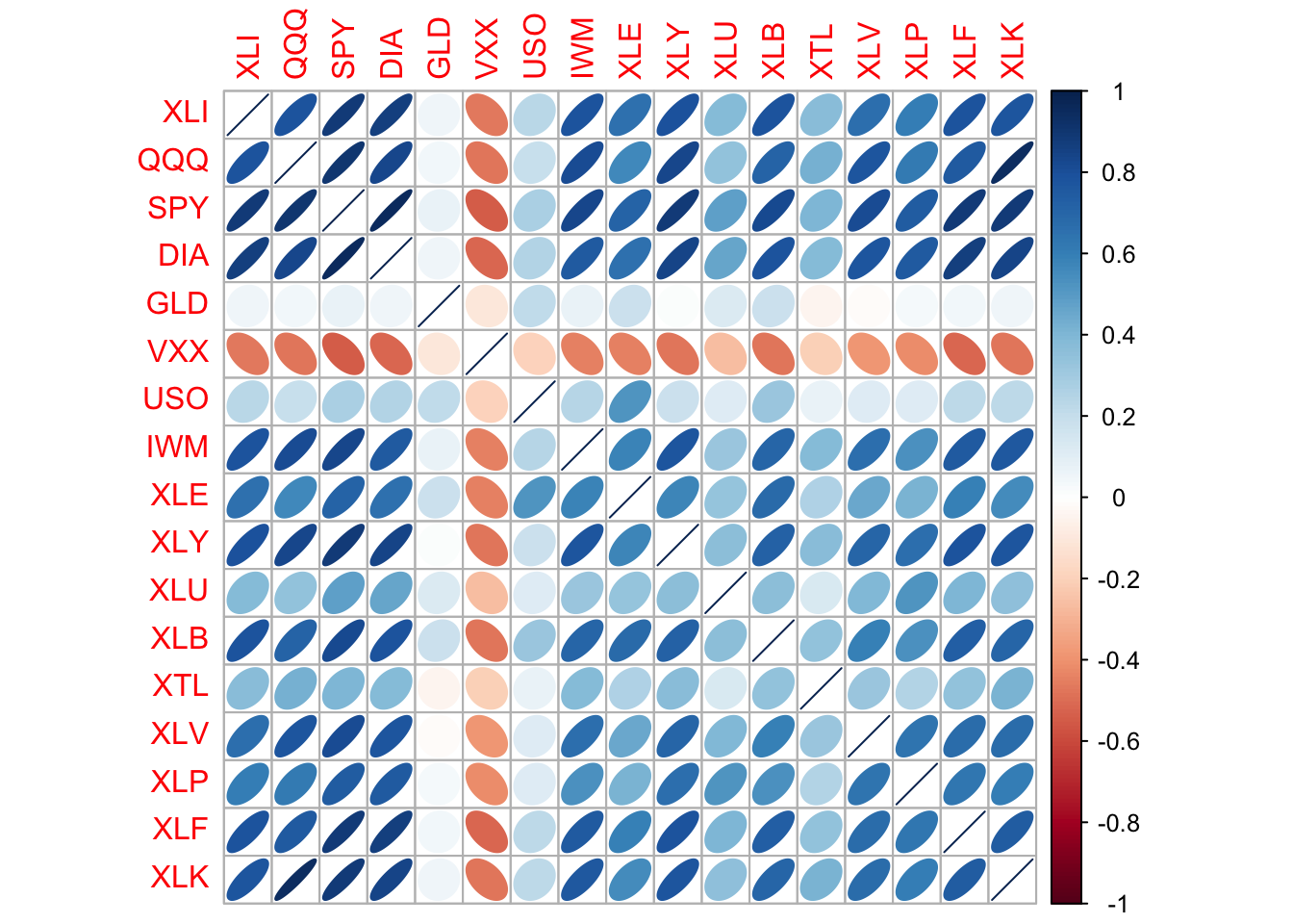

corrplot(cor(etfs), method = "ellipse")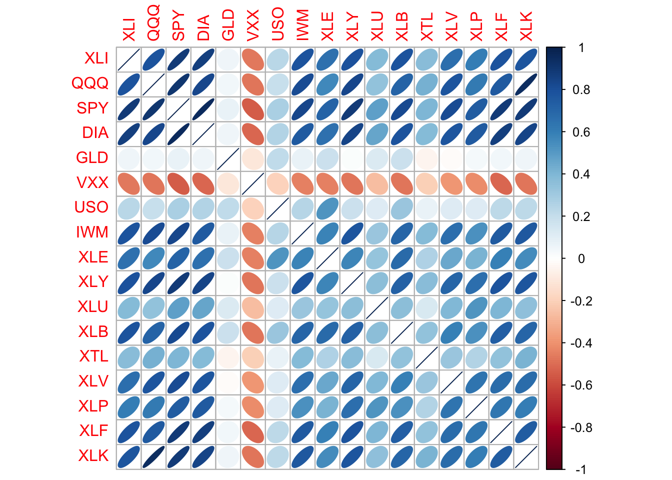

Scatterplots

ggplot(sp500_px %>% filter(Date > "2012-07-01"), aes(x = T, y = VZ)) +
  geom_point(shape = 1) +
  labs(x = "ATT (T)", y = "Verizon (VZ)")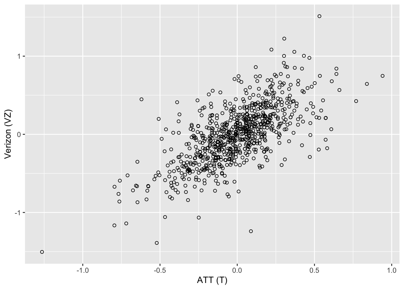

Exploring Two or More Variables

Hexagonal Binning and Contours pass:[<span class#“keep-together”>(Plotting Numeric-Versus-Numeric Data)]

kc_tax <- read_csv(file.path(DATA_DIR, "kc_tax.csv.gz"), show_col_types = FALSE)
kc_tax0 <- kc_tax %>%
  filter(TaxAssessedValue < 750000,
    SqFtTotLiving > 100,
    SqFtTotLiving < 3500)
nrow(kc_tax0)

[1] 432693

ggplot(kc_tax0, (aes(x = SqFtTotLiving, y = TaxAssessedValue))) +
  geom_hex(color = "white") +
  scale_fill_gradient(low = "white", high = "black") +
  labs(x = "Finished Square Feet", y = "Tax-Assessed Value")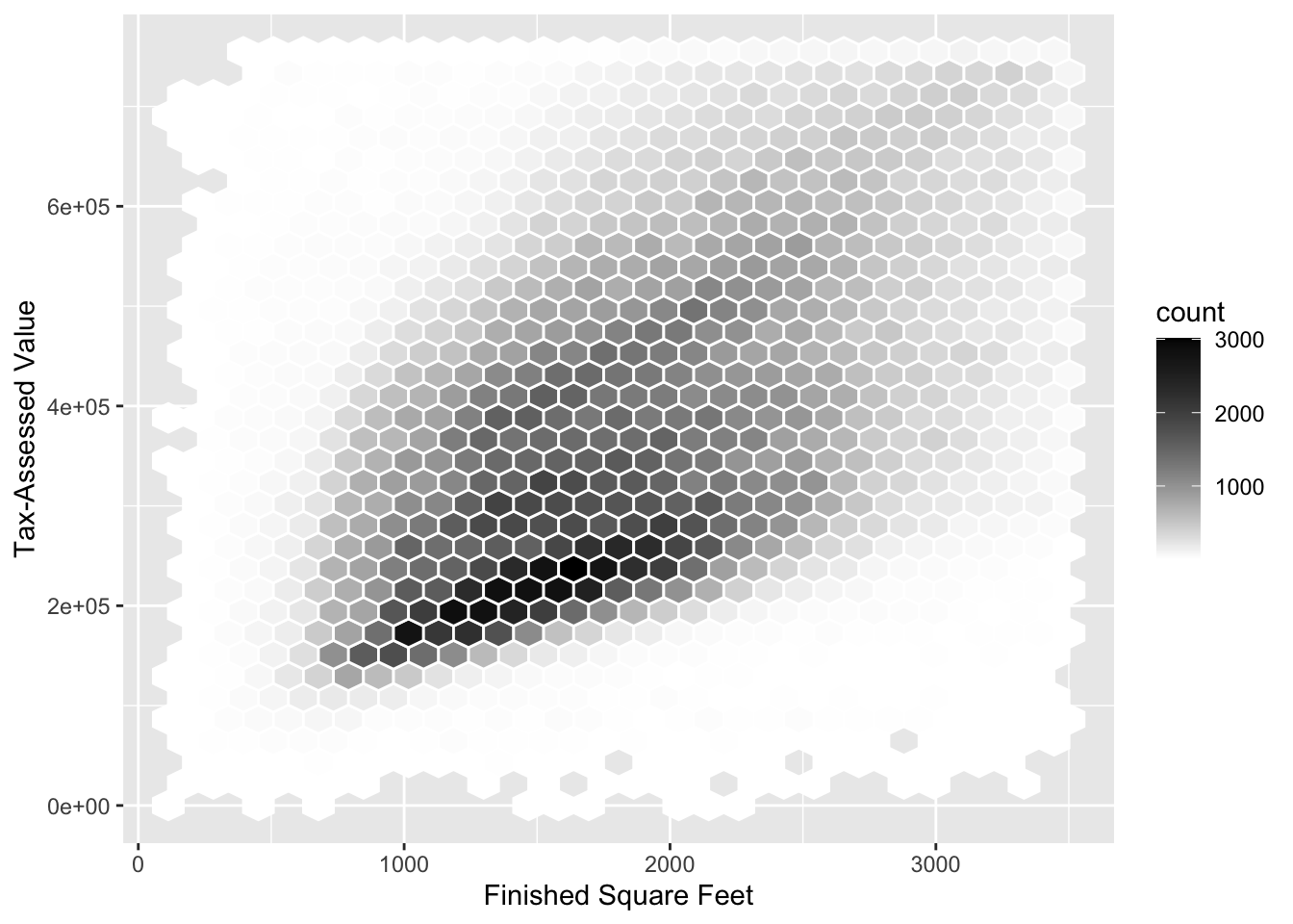

ggplot(kc_tax0, aes(SqFtTotLiving, TaxAssessedValue)) +
  geom_point(shape = 1, alpha = 0.02) +
  geom_density2d(color = "white") +
  labs(x = "Finished Square Feet", y = "Tax-Assessed Value")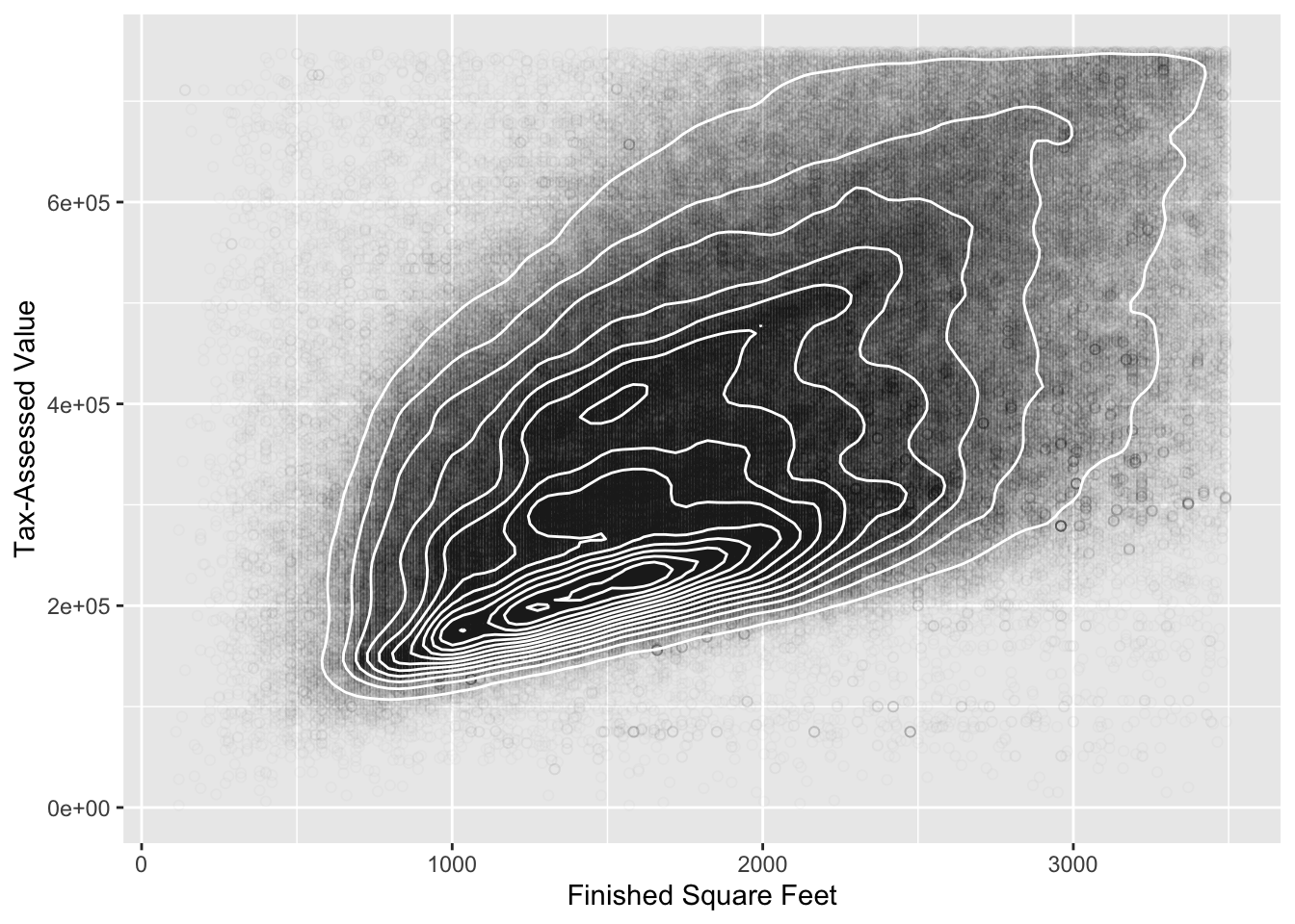

Two Categorical Variables

lc_loans <- read_csv(file.path(DATA_DIR, "lc_loans.csv"), show_col_types = FALSE)
x_tab <- CrossTable(lc_loans$grade, lc_loans$status,
  prop.c = FALSE, prop.chisq = FALSE, prop.t = FALSE)

 
   Cell Contents
|-------------------------|
|                       N |
|           N / Row Total |
|-------------------------|

 
Total Observations in Table:  450961 

 
               | lc_loans$status 
lc_loans$grade | Charged Off |     Current |  Fully Paid |        Late |   Row Total | 
---------------|-------------|-------------|-------------|-------------|-------------|
             A |        1562 |       50051 |       20408 |         469 |       72490 | 
               |       0.022 |       0.690 |       0.282 |       0.006 |       0.161 | 
---------------|-------------|-------------|-------------|-------------|-------------|
             B |        5302 |       93852 |       31160 |        2056 |      132370 | 
               |       0.040 |       0.709 |       0.235 |       0.016 |       0.294 | 
---------------|-------------|-------------|-------------|-------------|-------------|
             C |        6023 |       88928 |       23147 |        2777 |      120875 | 
               |       0.050 |       0.736 |       0.191 |       0.023 |       0.268 | 
---------------|-------------|-------------|-------------|-------------|-------------|
             D |        5007 |       53281 |       13681 |        2308 |       74277 | 
               |       0.067 |       0.717 |       0.184 |       0.031 |       0.165 | 
---------------|-------------|-------------|-------------|-------------|-------------|
             E |        2842 |       24639 |        5949 |        1374 |       34804 | 
               |       0.082 |       0.708 |       0.171 |       0.039 |       0.077 | 
---------------|-------------|-------------|-------------|-------------|-------------|
             F |        1526 |        8444 |        2328 |         606 |       12904 | 
               |       0.118 |       0.654 |       0.180 |       0.047 |       0.029 | 
---------------|-------------|-------------|-------------|-------------|-------------|
             G |         409 |        1990 |         643 |         199 |        3241 | 
               |       0.126 |       0.614 |       0.198 |       0.061 |       0.007 | 
---------------|-------------|-------------|-------------|-------------|-------------|
  Column Total |       22671 |      321185 |       97316 |        9789 |      450961 | 
---------------|-------------|-------------|-------------|-------------|-------------|

 

# Alternative to create crosstable using tidyverse
crosstab <- lc_loans  %>%
  group_by(status, grade) %>%
  count() %>%  # adds column n with the size of each group
  pivot_wider(id_cols = grade, names_from = status, values_from = n)
crosstab

# A tibble: 7 × 5
# Groups:   grade [7]
  grade `Charged Off` Current `Fully Paid`  Late
  <chr>         <int>   <int>        <int> <int>
1 A              1562   50051        20408   469
2 B              5302   93852        31160  2056
3 C              6023   88928        23147  2777
4 D              5007   53281        13681  2308
5 E              2842   24639         5949  1374
6 F              1526    8444         2328   606
7 G               409    1990          643   199

Categorical and Numeric Data

airline_stats <- read_csv(file.path(DATA_DIR, "airline_stats.csv"), show_col_types = FALSE) %>%
  mutate(
    airline = factor(airline,
      levels = c("Alaska", "American", "JetBlue", "Delta", "United",
        "Southwest"))
  ) %>%
  drop_na()

ggplot(airline_stats, aes(x = airline, y = pct_carrier_delay)) +
  geom_boxplot() +
  coord_cartesian(ylim = c(0, 50)) +
  labs(x = "Airline", y = "Daily % of Delayed Flights")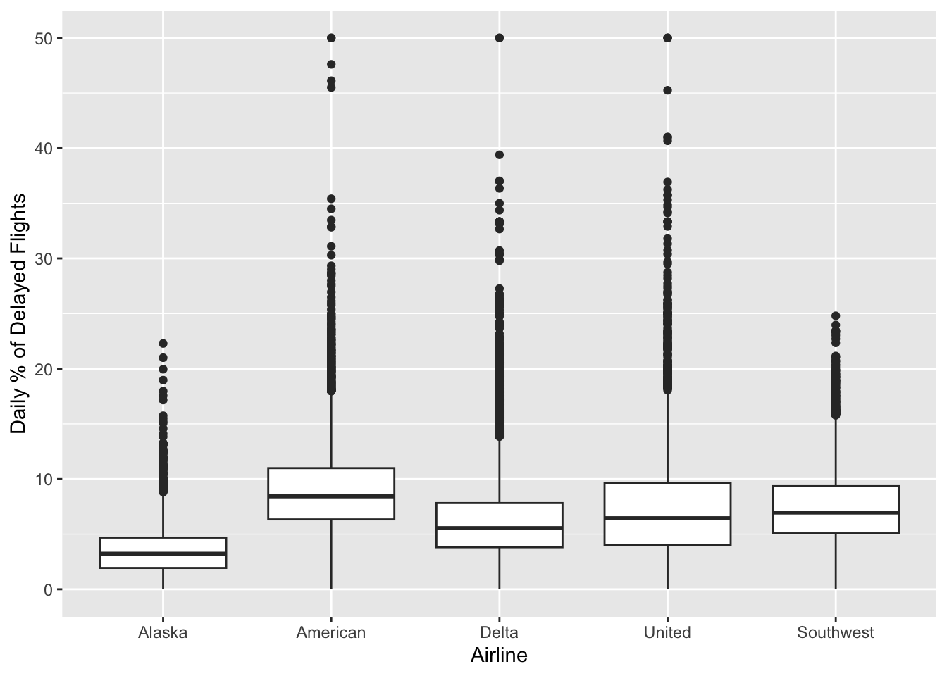

ggplot(data = airline_stats, aes(airline, pct_carrier_delay)) +
  geom_violin() +
  coord_cartesian(ylim = c(0, 50)) +
  labs(x = "", y = "Daily % of Delayed Flights")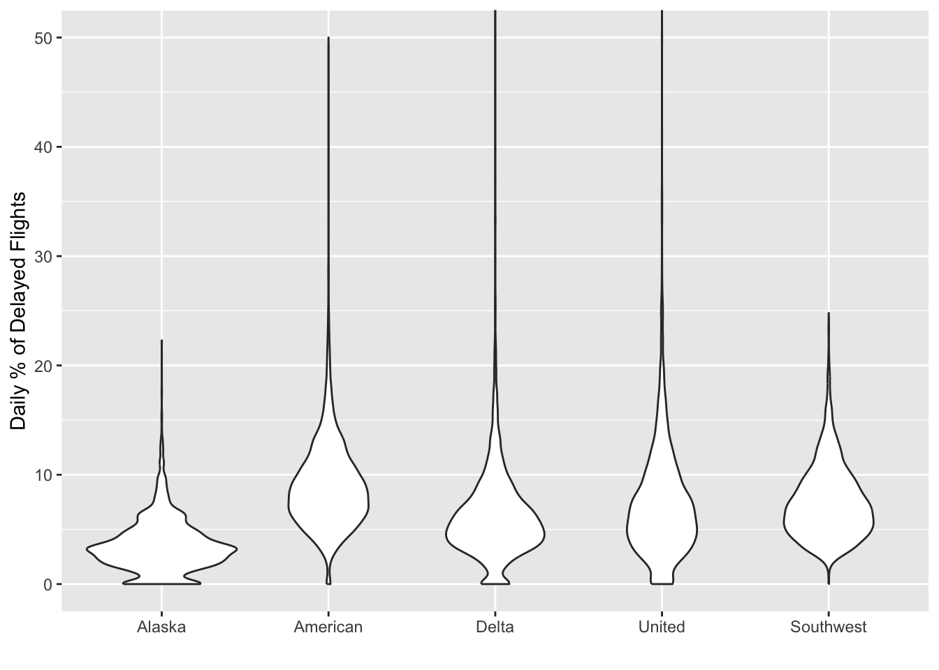

Visualizing Multiple Variables

kc_subset <- kc_tax0 %>%
  filter(ZipCode %in% c(98188, 98105, 98108, 98126))
ggplot(kc_subset, aes(x = SqFtTotLiving, y = TaxAssessedValue)) +
  geom_hex(color = "white") +
  scale_fill_gradient(low = "white", high = "blue") +
  labs(x = "Finished Square Feet", y = "Tax-Assessed Value") +
  facet_wrap("ZipCode")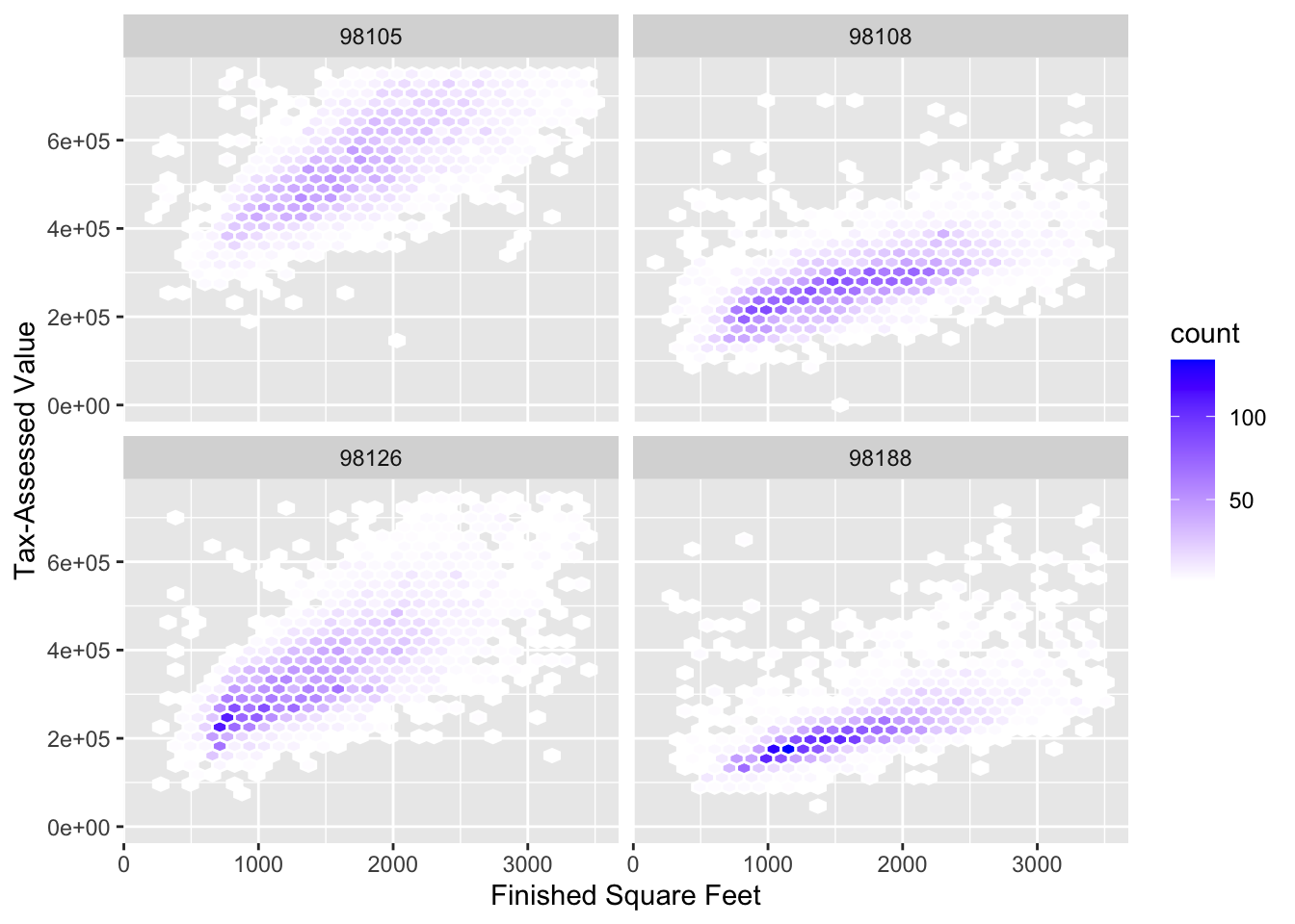

Supplementary Material

Table 1-2. A few rows of the data.frame state of population and murder rate by state

state %>%
  mutate(
    Population = formatC(Population, format = "d", digits = 0, big.mark = ","),
  ) %>%
  head(8)

# A tibble: 8 × 4
  State       Population Murder.Rate Abbreviation
  <chr>       <chr>            <dbl> <chr>       
1 Alabama     4,779,736          5.7 AL          
2 Alaska      710,231            5.6 AK          
3 Arizona     6,392,017          4.7 AZ          
4 Arkansas    2,915,918          5.6 AR          
5 California  37,253,956         4.4 CA          
6 Colorado    5,029,196          2.8 CO          
7 Connecticut 3,574,097          2.4 CT          
8 Delaware    897,934            5.8 DE          

Table 1-4. Percentiles of murder rate by state

Table 1-5. A frequency table of population by state

Table 1-6. Percentage of delays by cause at Dallas/Fort Worth Airport

Table 1-7. Correlation between telecommunication stock returns

Figure 1-6. Correlation between ETF returns (Python version)

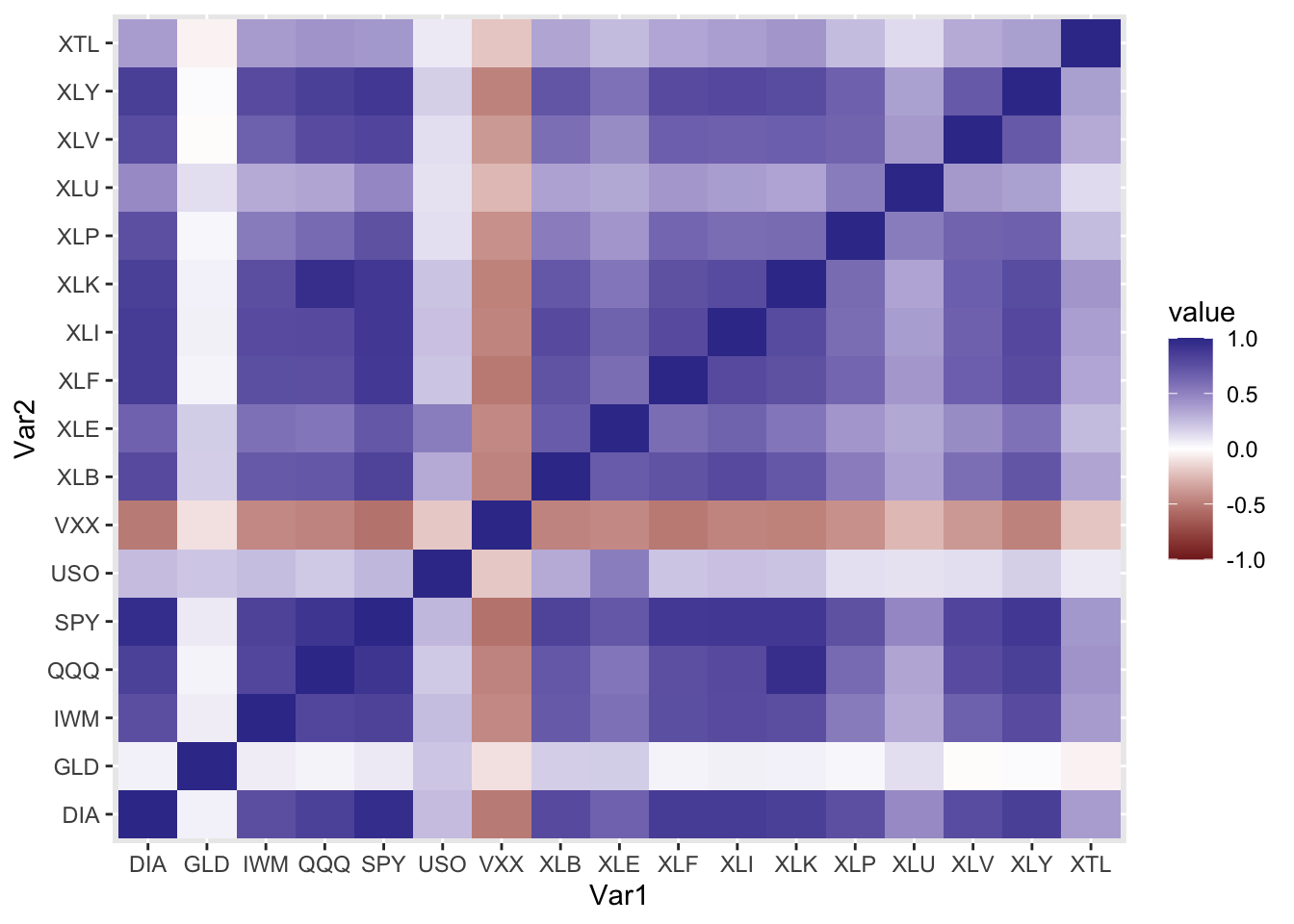
Figure 1-6. Correlation between ETF returns using a heat map (R version)

sp500_px <- read_csv(file.path(DATA_DIR, "sp500_data.csv.gz"), show_col_types = FALSE)
sp500_sym <- read_csv(file.path(DATA_DIR, "sp500_sectors.csv"), show_col_types = FALSE)
etf_symbols <- sp500_sym %>%
  filter(sector == "etf") %>%
  pull(symbol)
etfs <- sp500_px %>%
  filter(Date > "2012-07-01") %>%
  select(all_of(etf_symbols))
correlation_matrix <- cor(etfs) %>%
  as_tibble() %>%
  mutate(Var1 = colnames(.)) %>%
  pivot_longer(-Var1, names_to = "Var2", values_to = "value")

ggplot(correlation_matrix, aes(x = Var1, y = Var2)) +
  geom_tile(aes(fill = value)) +
  scale_fill_gradient2(limits = c(-1, 1))