library(boot)
library(tidyverse)

set.seed(123)

# Location of the data files. Adjust this path if you keep the data
# files in a different directory.
DATA_DIR <- '../data'Chapter 2: Data and Sampling Distributions
Data and Sampling Distributions
Sampling Distribution of a Statistic
loans_income <- read_csv(file.path(DATA_DIR, "loans_income.csv"), show_col_types = FALSE) %>%
  pull(x)

# take a simple random sample
samp_data <- data.frame(income = sample(loans_income, 1000),
  type = "Data")
# take a sample of means of 5 values
samp_mean_05 <- tibble(
  income = replicate(1000, mean(sample(loans_income, 5))),
  type = "Mean of 5"
)
# take a sample of means of 20 values
samp_mean_20 <- tibble(
  income = replicate(1000, mean(sample(loans_income, 20))),
  type = "Mean of 20"
)
income <- bind_rows(samp_data, samp_mean_05, samp_mean_20) %>%
  mutate(type = factor(type,
      levels = c("Data", "Mean of 5", "Mean of 20"))
  )

# plot the histograms
ggplot(income, aes(x = income)) +
  geom_histogram(bins = 40) +
  facet_grid(type ~ .)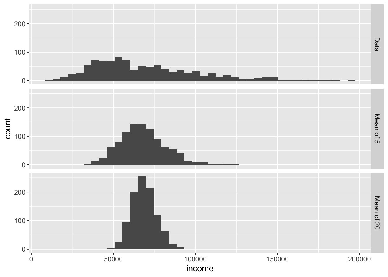
The Bootstrap
stat_fun <- function(x, idx) median(x[idx])
boot_obj <- boot(loans_income, R = 1000, statistic = stat_fun)
boot_obj
ORDINARY NONPARAMETRIC BOOTSTRAP


Call:
boot(data = loans_income, statistic = stat_fun, R = 1000)


Bootstrap Statistics :
    original   bias    std. error
t1*    62000 -78.0335     218.435
Normal Distribution
Standard Normal and QQ-Plots
norm_samp <- rnorm(100)
ggplot(tibble(y = norm_samp), aes(sample = y)) +
  geom_qq() +
  geom_qq_line() +
  labs(x = "Theoretical Quantiles", y = "Sample Quantiles")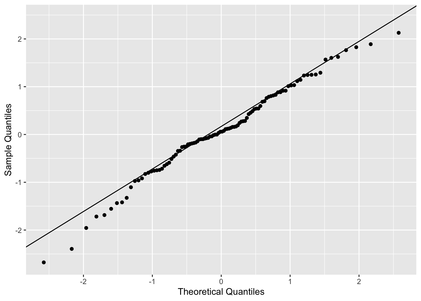
# alternative using qqnorm
qqnorm(norm_samp)
qqline(norm_samp)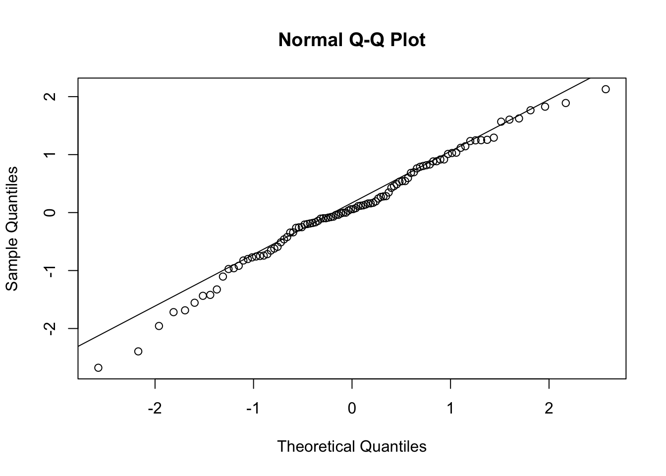
Long-Tailed Distributions
sp500_px <- read_csv(file.path(DATA_DIR, "sp500_data.csv.gz"), show_col_types = FALSE)

nflx <- sp500_px[, "NFLX"]
nflx <- diff(log(nflx[nflx > 0]))
qqnorm(nflx)
abline(a = 0, b = 1, col = "grey")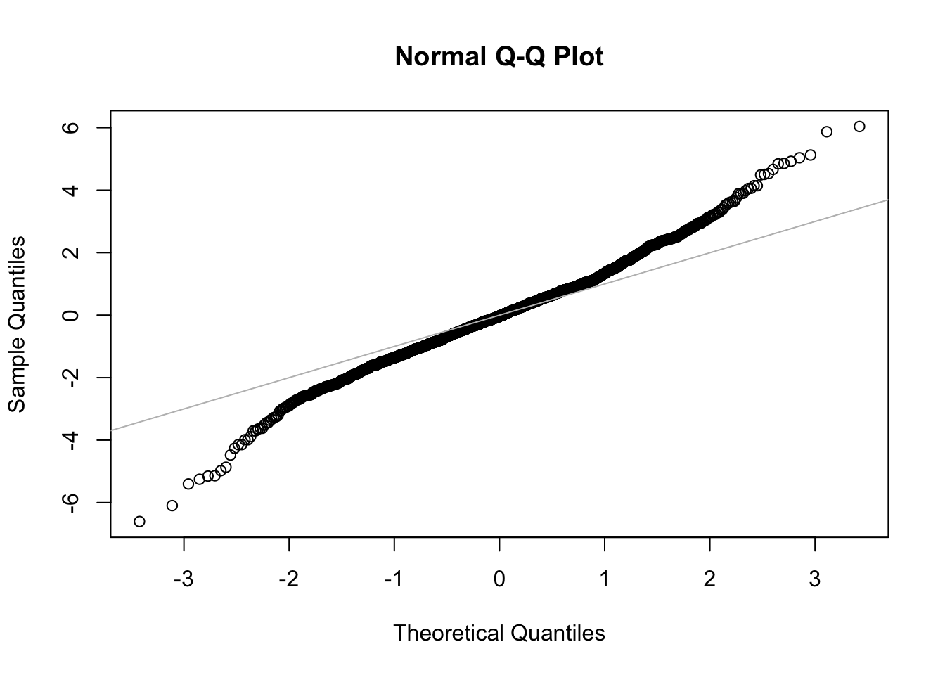
ggplot(tibble(y = nflx), aes(sample = y)) +
  geom_qq() +
  geom_qq_line() +
  labs(x = "Theoretical Quantiles", y = "Sample Quantiles")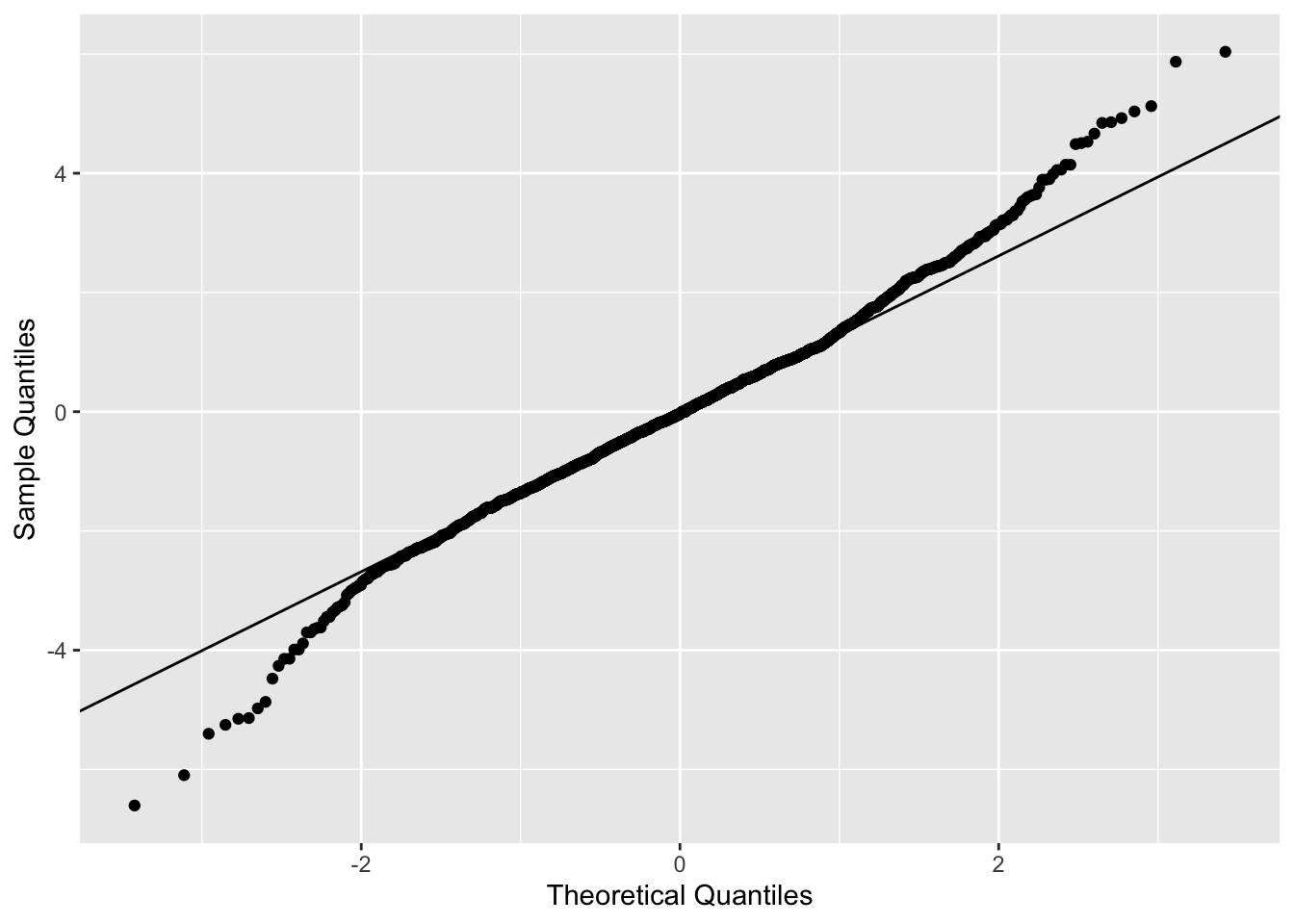
Binomial Distribution
dbinom(x = 2, size = 5, prob = 0.1)[1] 0.0729pbinom(q = 2, size = 5, prob = 0.1)[1] 0.99144Supplementary Material
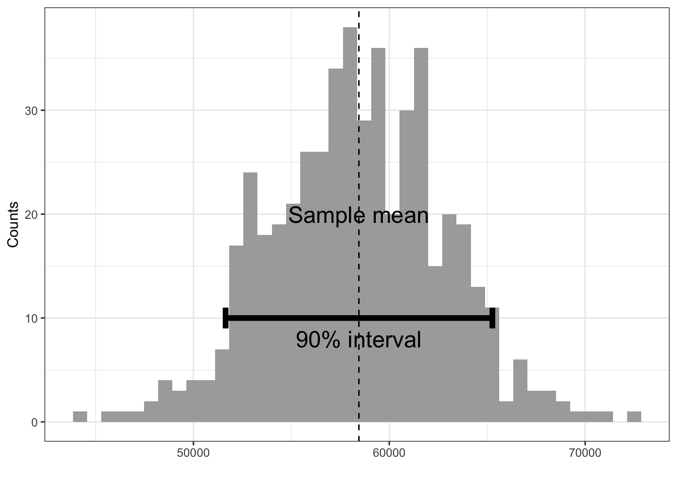
Figure 2-9 Bootstrap confidence interval for the annual income of loan applicants, based on a sample of 20
loans_income <- read_csv(file.path(DATA_DIR, "loans_income.csv"), show_col_types = FALSE) %>%
  pull(x)

set.seed(7)
sample20 <- sample(loans_income, 20)
sample_mean <- mean(sample20)

stat_fun <- function(x, idx) mean(x[idx])
boot_obj <- boot(sample20, R = 500, statistic = stat_fun)
boot_ci <- boot.ci(boot_obj, conf = 0.9, type = "basic")
df <- data.frame(mean = boot_obj$t)
ci90 <- boot_ci$basic[4:5]
ci <- data.frame(ci = ci90, y = c(9, 11))
ci
ci y
1 51643.09 9
2 65262.95 11ggplot(df, aes(x = mean)) +
geom_histogram(bins = 40, fill = "#AAAAAA") +
geom_vline(xintercept = sample_mean, linetype = 2) +
geom_path(aes(x = ci, y = 10), data = ci, linewidth = 2) +
geom_path(aes(x = ci90[1], y = y), data = ci, linewidth = 2) +
geom_path(aes(x = ci90[2], y = y), data = ci, linewidth = 2) +
annotate("text", x = sample_mean, y = 20, label = "Sample mean", size = 6) +
annotate("text", x = sample_mean, y = 8, label = "90% interval", size = 6) +
theme_bw() +
labs(x = "", y = "Counts")