library(MASS)
library(latex2exp)
library(lubridate)
library(mgcv)
library(splines)
library(tidyverse)

set.seed(123)

# Location of the data files. Adjust this path if you keep the data
# files in a different directory.
DATA_DIR <- '../data'Chapter 4: Regression and Prediction
Regression and Prediction
Simple Linear Regression
The Regression Equation
lung <- read_csv(file.path(DATA_DIR, "LungDisease.csv"))Rows: 122 Columns: 2
── Column specification ────────────────────────────────────────────────────────
Delimiter: ","
dbl (2): PEFR, Exposure
ℹ Use `spec()` to retrieve the full column specification for this data.
ℹ Specify the column types or set `show_col_types = FALSE` to quiet this message.model <- lm(PEFR ~ Exposure, data = lung)PEFR ~ Exposure - 1PEFR ~ Exposure - 1model
Call:
lm(formula = PEFR ~ Exposure, data = lung)

Coefficients:
(Intercept)     Exposure
    424.583       -4.185
Fitted Values and Residuals
fitted <- predict(model)
resid <- residuals(model)
Multiple Linear Regression
Example: King County Housing Data
house <- read_csv(file.path(DATA_DIR, "house_sales.csv"), show_col_types = FALSE)
head(house[, c("AdjSalePrice", "SqFtTotLiving", "SqFtLot", "Bathrooms",
      "Bedrooms", "BldgGrade")])
# A tibble: 6 × 6
AdjSalePrice SqFtTotLiving SqFtLot Bathrooms Bedrooms BldgGrade
<dbl> <dbl> <dbl> <dbl> <dbl> <dbl>
1 300805 2400 9373 3 6 7
2 1076162 3764 20156 3.75 4 10
3 761805 2060 26036 1.75 4 8
4 442065 3200 8618 3.75 5 7
5 297065 1720 8620 1.75 4 7
6 411781 930 1012 1.5 2 8house_lm <- lm(AdjSalePrice ~ SqFtTotLiving + SqFtLot + Bathrooms +
Bedrooms + BldgGrade,
data = house, na.action = na.omit)house_lm
Call:
lm(formula = AdjSalePrice ~ SqFtTotLiving + SqFtLot + Bathrooms +
    Bedrooms + BldgGrade, data = house, na.action = na.omit)

Coefficients:
  (Intercept)  SqFtTotLiving        SqFtLot      Bathrooms       Bedrooms
   -5.219e+05      2.288e+02     -6.047e-02     -1.944e+04     -4.777e+04
    BldgGrade
    1.061e+05
Assessing the Model
summary(house_lm)
Call:
lm(formula = AdjSalePrice ~ SqFtTotLiving + SqFtLot + Bathrooms +
    Bedrooms + BldgGrade, data = house, na.action = na.omit)

Residuals:
     Min       1Q   Median       3Q      Max
-1199479  -118908   -20977    87435  9473035

Coefficients:
                Estimate Std. Error t value Pr(>|t|)
(Intercept)   -5.219e+05  1.565e+04 -33.342  < 2e-16 ***
SqFtTotLiving  2.288e+02  3.899e+00  58.694  < 2e-16 ***
SqFtLot       -6.047e-02  6.118e-02  -0.988    0.323
Bathrooms     -1.944e+04  3.625e+03  -5.363 8.27e-08 ***
Bedrooms      -4.777e+04  2.490e+03 -19.187  < 2e-16 ***
BldgGrade      1.061e+05  2.396e+03  44.277  < 2e-16 ***
---
Signif. codes:  0 '***' 0.001 '**' 0.01 '*' 0.05 '.' 0.1 ' ' 1

Residual standard error: 261300 on 22681 degrees of freedom
Multiple R-squared:  0.5406,    Adjusted R-squared:  0.5405
F-statistic:  5338 on 5 and 22681 DF,  p-value: < 2.2e-16
Model Selection and Stepwise Regression
house_full <- lm(AdjSalePrice ~ SqFtTotLiving + SqFtLot + Bathrooms +
    Bedrooms + BldgGrade + PropertyType + NbrLivingUnits +
    SqFtFinBasement + YrBuilt + YrRenovated + NewConstruction,
  data = house, na.action = na.omit)
step_lm <- stepAIC(house_full, direction = "both")Start: AIC=563145.4
AdjSalePrice ~ SqFtTotLiving + SqFtLot + Bathrooms + Bedrooms +
BldgGrade + PropertyType + NbrLivingUnits + SqFtFinBasement +
YrBuilt + YrRenovated + NewConstruction
Df Sum of Sq RSS AIC
- NbrLivingUnits 1 6.4007e+09 1.3662e+15 563144
- NewConstruction 1 1.0592e+10 1.3662e+15 563144
- YrRenovated 1 2.5069e+10 1.3662e+15 563144
- SqFtLot 1 1.0657e+11 1.3663e+15 563145
<none> 1.3662e+15 563145
- SqFtFinBasement 1 1.4030e+11 1.3663e+15 563146
- PropertyType 2 4.4207e+12 1.3706e+15 563215
- Bathrooms 1 7.6325e+12 1.3738e+15 563270
- Bedrooms 1 2.8212e+13 1.3944e+15 563607
- YrBuilt 1 1.2906e+14 1.4952e+15 565191
- SqFtTotLiving 1 1.3264e+14 1.4988e+15 565246
- BldgGrade 1 1.9050e+14 1.5567e+15 566105
Step: AIC=563143.6
AdjSalePrice ~ SqFtTotLiving + SqFtLot + Bathrooms + Bedrooms +
BldgGrade + PropertyType + SqFtFinBasement + YrBuilt + YrRenovated +
NewConstruction
Df Sum of Sq RSS AIC
- NewConstruction 1 1.0801e+10 1.3662e+15 563142
- YrRenovated 1 2.5628e+10 1.3662e+15 563142
- SqFtLot 1 1.0731e+11 1.3663e+15 563143
<none> 1.3662e+15 563144
- SqFtFinBasement 1 1.3828e+11 1.3663e+15 563144
+ NbrLivingUnits 1 6.4007e+09 1.3662e+15 563145
- PropertyType 2 4.4301e+12 1.3706e+15 563213
- Bathrooms 1 7.7500e+12 1.3739e+15 563270
- Bedrooms 1 2.8273e+13 1.3944e+15 563606
- YrBuilt 1 1.3013e+14 1.4963e+15 565206
- SqFtTotLiving 1 1.3288e+14 1.4990e+15 565247
- BldgGrade 1 1.9177e+14 1.5579e+15 566122
Step: AIC=563141.7
AdjSalePrice ~ SqFtTotLiving + SqFtLot + Bathrooms + Bedrooms +
BldgGrade + PropertyType + SqFtFinBasement + YrBuilt + YrRenovated
Df Sum of Sq RSS AIC
- YrRenovated 1 2.5893e+10 1.3662e+15 563140
- SqFtLot 1 1.1494e+11 1.3663e+15 563142
<none> 1.3662e+15 563142
- SqFtFinBasement 1 1.4534e+11 1.3663e+15 563142
+ NewConstruction 1 1.0801e+10 1.3662e+15 563144
+ NbrLivingUnits 1 6.6093e+09 1.3662e+15 563144
- PropertyType 2 4.5301e+12 1.3707e+15 563213
- Bathrooms 1 7.7487e+12 1.3739e+15 563268
- Bedrooms 1 2.8269e+13 1.3945e+15 563604
- SqFtTotLiving 1 1.3390e+14 1.5001e+15 565261
- YrBuilt 1 1.3760e+14 1.5038e+15 565317
- BldgGrade 1 1.9244e+14 1.5586e+15 566129
Step: AIC=563140.2
AdjSalePrice ~ SqFtTotLiving + SqFtLot + Bathrooms + Bedrooms +
BldgGrade + PropertyType + SqFtFinBasement + YrBuilt
Df Sum of Sq RSS AIC
- SqFtLot 1 1.1425e+11 1.3663e+15 563140
<none> 1.3662e+15 563140
- SqFtFinBasement 1 1.4999e+11 1.3664e+15 563141
+ YrRenovated 1 2.5893e+10 1.3662e+15 563142
+ NewConstruction 1 1.1065e+10 1.3662e+15 563142
+ NbrLivingUnits 1 7.1825e+09 1.3662e+15 563142
- PropertyType 2 4.5076e+12 1.3707e+15 563211
- Bathrooms 1 7.7790e+12 1.3740e+15 563267
- Bedrooms 1 2.8251e+13 1.3945e+15 563603
- SqFtTotLiving 1 1.3388e+14 1.5001e+15 565259
- YrBuilt 1 1.5091e+14 1.5171e+15 565515
- BldgGrade 1 1.9244e+14 1.5587e+15 566128
Step: AIC=563140.1
AdjSalePrice ~ SqFtTotLiving + Bathrooms + Bedrooms + BldgGrade +
PropertyType + SqFtFinBasement + YrBuilt
Df Sum of Sq RSS AIC
<none> 1.3663e+15 563140
+ SqFtLot 1 1.1425e+11 1.3662e+15 563140
- SqFtFinBasement 1 1.4116e+11 1.3665e+15 563140
+ YrRenovated 1 2.5199e+10 1.3663e+15 563142
+ NewConstruction 1 1.8750e+10 1.3663e+15 563142
+ NbrLivingUnits 1 8.0521e+09 1.3663e+15 563142
- PropertyType 2 4.4415e+12 1.3708e+15 563210
- Bathrooms 1 7.7109e+12 1.3740e+15 563266
- Bedrooms 1 2.8553e+13 1.3949e+15 563607
- SqFtTotLiving 1 1.3748e+14 1.5038e+15 565313
- YrBuilt 1 1.5080e+14 1.5171e+15 565513
- BldgGrade 1 1.9234e+14 1.5587e+15 566126step_lm
Call:
lm(formula = AdjSalePrice ~ SqFtTotLiving + Bathrooms + Bedrooms +
    BldgGrade + PropertyType + SqFtFinBasement + YrBuilt, data = house,
    na.action = na.omit)

Coefficients:
              (Intercept)              SqFtTotLiving
                6.179e+06                  1.993e+02
                Bathrooms                   Bedrooms
                4.240e+04                 -5.195e+04
                BldgGrade  PropertyTypeSingle Family
                1.372e+05                  2.291e+04
    PropertyTypeTownhouse            SqFtFinBasement
                8.448e+04                  7.047e+00
                  YrBuilt
               -3.565e+03
Weighted Regression
house$Year <- year(parse_date_time(house$DocumentDate, "m/d/y"))
house$Weight <- house$Year - 2005
house_wt <- lm(AdjSalePrice ~ SqFtTotLiving + SqFtLot + Bathrooms +
Bedrooms + BldgGrade,
data = house, weight = Weight)
round(cbind(house_lm = house_lm$coefficients,
house_wt = house_wt$coefficients), digits = 3) house_lm house_wt
(Intercept) -521871.368 -584189.329
SqFtTotLiving 228.831 245.024
SqFtLot -0.060 -0.292
Bathrooms -19442.840 -26085.970
Bedrooms -47769.955 -53608.876
BldgGrade 106106.963 115242.435Factor Variables in Regression
Dummy Variables Representation
head(house[, "PropertyType"])# A tibble: 6 × 1
PropertyType
<chr>
1 Multiplex
2 Single Family
3 Single Family
4 Single Family
5 Single Family
6 Townhouse prop_type_dummies <- model.matrix(~ PropertyType - 1, data = house)
head(prop_type_dummies) PropertyTypeMultiplex PropertyTypeSingle Family PropertyTypeTownhouse
1 1 0 0
2 0 1 0
3 0 1 0
4 0 1 0
5 0 1 0
6 0 0 1lm(AdjSalePrice ~ SqFtTotLiving + SqFtLot + Bathrooms +
Bedrooms + BldgGrade + PropertyType, data = house)
Call:
lm(formula = AdjSalePrice ~ SqFtTotLiving + SqFtLot + Bathrooms +
    Bedrooms + BldgGrade + PropertyType, data = house)

Coefficients:
              (Intercept)              SqFtTotLiving
               -4.468e+05                  2.234e+02
                  SqFtLot                  Bathrooms
               -7.037e-02                 -1.598e+04
                 Bedrooms                  BldgGrade
               -5.089e+04                  1.094e+05
PropertyTypeSingle Family      PropertyTypeTownhouse
               -8.468e+04                 -1.151e+05
Factor Variables with Many Levels
table(house$ZipCode)
98001 98002 98003 98004 98005 98006 98007 98008 98010 98011 98014 98019 98022
  358   180   241   293   133   460   112   291    56   163    85   242   188
98023 98024 98027 98028 98029 98030 98031 98032 98033 98034 98038 98039 98040
  455    31   366   252   475   263   308   121   517   575   788    47   244
98042 98043 98045 98047 98050 98051 98052 98053 98055 98056 98057 98058 98059
  641     1   222    48     7    32   614   499   332   402     4   420   513
98065 98068 98070 98072 98074 98075 98077 98092 98102 98103 98105 98106 98107
  430     1    89   245   502   388   204   289   106   671   313   361   296
98108 98109 98112 98113 98115 98116 98117 98118 98119 98122 98125 98126 98133
  155   149   357     1   620   364   619   492   260   380   409   473   465
98136 98144 98146 98148 98155 98166 98168 98177 98178 98188 98198 98199 98224
  310   332   287    40   358   193   332   216   266   101   225   393     3
98288 98354
    4     9
zip_groups <- house %>%
mutate(resid = residuals(house_lm)) %>%
group_by(ZipCode) %>%
summarize(med_resid = median(resid), cnt = n()) %>%
arrange(med_resid) %>%
mutate(
cum_cnt = cumsum(cnt),
ZipGroup = ntile(cum_cnt, 5),
) %>%
select(ZipCode, ZipGroup)
house <- house %>%
left_join(zip_groups, by = "ZipCode") %>%
mutate(ZipGroup = as.factor(ZipGroup))table(zip_groups[c("ZipGroup")])ZipGroup
1 2 3 4 5
16 16 16 16 16 Interpreting the Regression Equation
Confounding Variables
lm(AdjSalePrice ~ SqFtTotLiving + SqFtLot + Bathrooms +
    Bedrooms + BldgGrade + PropertyType + ZipGroup, data = house,
  na.action = na.omit)
Call:
lm(formula = AdjSalePrice ~ SqFtTotLiving + SqFtLot + Bathrooms +
    Bedrooms + BldgGrade + PropertyType + ZipGroup, data = house,
    na.action = na.omit)

Coefficients:
              (Intercept)              SqFtTotLiving
               -6.666e+05                  2.106e+02
                  SqFtLot                  Bathrooms
                4.550e-01                  5.928e+03
                 Bedrooms                  BldgGrade
               -4.168e+04                  9.854e+04
PropertyTypeSingle Family      PropertyTypeTownhouse
                1.932e+04                 -7.820e+04
                ZipGroup2                  ZipGroup3
                5.332e+04                  1.163e+05
                ZipGroup4                  ZipGroup5
                1.784e+05                  3.384e+05
Interactions and Main Effects
lm(formula = AdjSalePrice ~ SqFtTotLiving * ZipGroup + SqFtLot +
    Bathrooms + Bedrooms + BldgGrade + PropertyType, data = house,
  na.action = na.omit)
Call:
lm(formula = AdjSalePrice ~ SqFtTotLiving * ZipGroup + SqFtLot +
    Bathrooms + Bedrooms + BldgGrade + PropertyType, data = house,
    na.action = na.omit)

Coefficients:
              (Intercept)              SqFtTotLiving
               -4.853e+05                  1.148e+02
                ZipGroup2                  ZipGroup3
               -1.113e+04                  2.032e+04
                ZipGroup4                  ZipGroup5
                2.050e+04                 -1.499e+05
                  SqFtLot                  Bathrooms
                6.869e-01                 -3.619e+03
                 Bedrooms                  BldgGrade
               -4.180e+04                  1.047e+05
PropertyTypeSingle Family      PropertyTypeTownhouse
                1.357e+04                 -5.884e+04
  SqFtTotLiving:ZipGroup2    SqFtTotLiving:ZipGroup3
                3.260e+01                  4.178e+01
  SqFtTotLiving:ZipGroup4    SqFtTotLiving:ZipGroup5
                6.934e+01                  2.267e+02
Regression Diagnostics
Outliers
house_98105 <- house %>% filter(ZipCode == 98105)
lm_98105 <- lm(AdjSalePrice ~ SqFtTotLiving + SqFtLot + Bathrooms +
    Bedrooms + BldgGrade, data = house_98105)
sresid <- rstandard(lm_98105)
idx <- order(sresid)
sresid[idx[1]] 259
-4.326732 house_98105[idx[1], c("AdjSalePrice", "SqFtTotLiving", "SqFtLot",
"Bathrooms", "Bedrooms", "BldgGrade")]# A tibble: 1 × 6
AdjSalePrice SqFtTotLiving SqFtLot Bathrooms Bedrooms BldgGrade
<dbl> <dbl> <dbl> <dbl> <dbl> <dbl>
1 119748 2900 7276 3 6 7Influential Values
df_influential <- tibble(
  std_resid = rstandard(lm_98105),
  cooks_d = cooks.distance(lm_98105),
  hat_values = hatvalues(lm_98105),
)

p <- 6 # Number of model parameters (e.g., intercept + 2 predictors)
D_i <- 0.08 # Target Cook's Distance
cooks_curve_data <- tibble(
  t = seq(-10, 10, length.out = 1000),
  cooks_d = 0.08,
) %>%
  mutate(
    hat_values = 1 / (1 + t^2),
    std_resid = sqrt(D_i * p) * t
  )

ggplot(df_influential, aes(x = hat_values, y = std_resid,
    color = cooks_d > 0.08, shape = cooks_d > 0.08)) +
  geom_path(aes(size = NULL, color = NULL, shape = NULL),
    data = cooks_curve_data, color = "grey", linewidth = 0.5) +
  geom_hline(yintercept = c(-2.5, 2.5), linetype = 2) +
  geom_point(aes(size = 10 * sqrt(cooks_d))) +
  scale_shape_manual(values = c(1, 19)) +
  guides(color = "none", shape = "none", size = "none") +
  coord_cartesian(xlim = c(0, 0.3), ylim = c(-6, 6), expand = FALSE)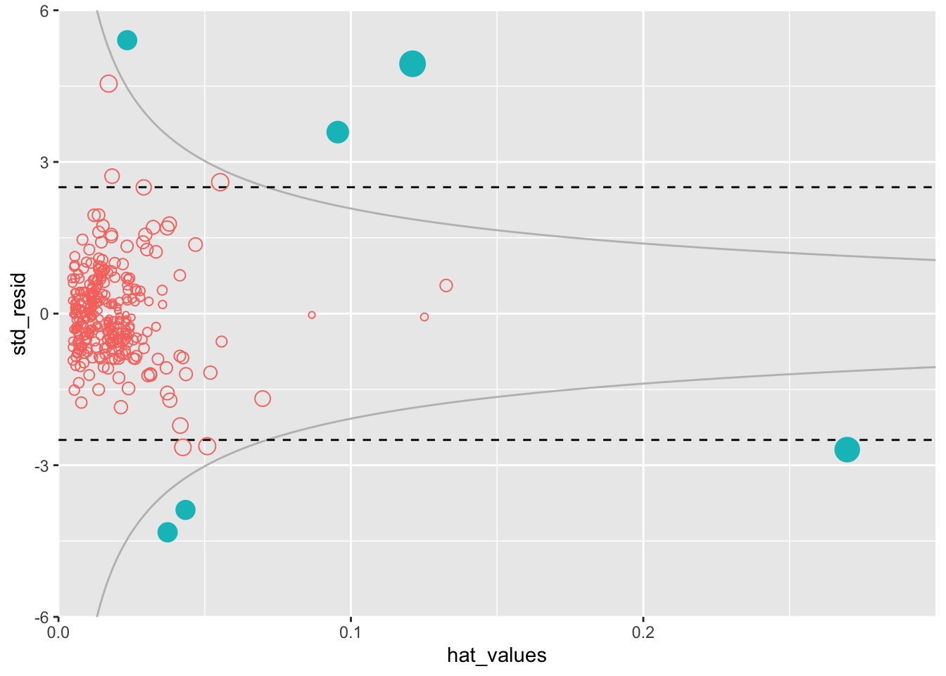
Heteroskedasticity, Nonnormality, and Correlated Errors
df <- data.frame(resid = residuals(lm_98105), pred = predict(lm_98105))
ggplot(df, aes(x = pred, y = abs(resid))) +
  geom_point() +
  geom_smooth(formula = y ~ x, method = "loess") +
  scale_x_continuous(labels = function(x) format(x, scientific = FALSE))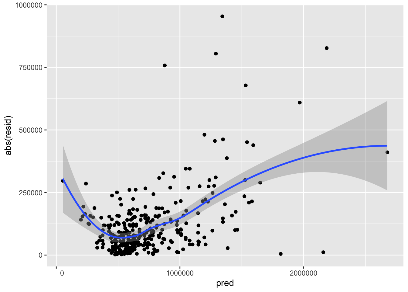
Partial Residual Plots and Nonlinearity
terms <- predict(lm_98105, type = "terms")
partial_resid <- resid(lm_98105) + terms
df <- data.frame(SqFtTotLiving = house_98105[, "SqFtTotLiving"],
Terms = terms[, "SqFtTotLiving"],
PartialResid = partial_resid[, "SqFtTotLiving"])
ggplot(df, aes(SqFtTotLiving, PartialResid)) +
geom_point(shape = 1) +
scale_shape(solid = FALSE) +
geom_smooth(linetype = 2) +
geom_line(aes(SqFtTotLiving, Terms))`geom_smooth()` using method = 'loess' and formula = 'y ~ x'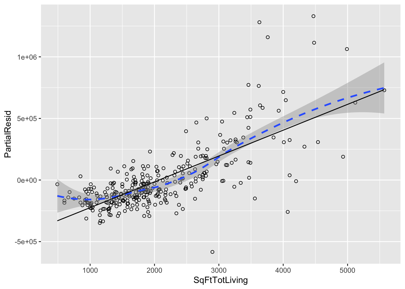
Polynomial and Spline Regression
Polynomial
lm_poly <- lm(AdjSalePrice ~ poly(SqFtTotLiving, 2) + SqFtLot +
    BldgGrade + Bathrooms + Bedrooms, data = house_98105)
lm_poly
Call:
lm(formula = AdjSalePrice ~ poly(SqFtTotLiving, 2) + SqFtLot +
    BldgGrade + Bathrooms + Bedrooms, data = house_98105)

Coefficients:
            (Intercept)  poly(SqFtTotLiving, 2)1  poly(SqFtTotLiving, 2)2
             -402530.47               3271519.49                776934.02
                SqFtLot                BldgGrade                Bathrooms
                  32.56                135717.06                 -1435.12
               Bedrooms
               -9191.94
Splines
knots <- quantile(house_98105$SqFtTotLiving, p = c(0.25, 0.5, 0.75))
lm_spline <- lm(AdjSalePrice ~ bs(SqFtTotLiving, knots = knots, degree = 3) +
    SqFtLot + Bathrooms + Bedrooms + BldgGrade,
  data = house_98105)
lm_spline
Call:
lm(formula = AdjSalePrice ~ bs(SqFtTotLiving, knots = knots,
    degree = 3) + SqFtLot + Bathrooms + Bedrooms + BldgGrade,
    data = house_98105)

Coefficients:
                                  (Intercept)
                                   -414157.61
bs(SqFtTotLiving, knots = knots, degree = 3)1
                                   -199529.76
bs(SqFtTotLiving, knots = knots, degree = 3)2
                                   -120580.64
bs(SqFtTotLiving, knots = knots, degree = 3)3
                                    -71644.39
bs(SqFtTotLiving, knots = knots, degree = 3)4
                                    195677.89
bs(SqFtTotLiving, knots = knots, degree = 3)5
                                    845244.25
bs(SqFtTotLiving, knots = knots, degree = 3)6
                                    695545.67
                                      SqFtLot
                                        33.33
                                    Bathrooms
                                     -4778.21
                                     Bedrooms
                                     -5778.70
                                    BldgGrade
                                    134462.37
Generalized Additive Models
lm_gam <- gam(AdjSalePrice ~ s(SqFtTotLiving) + SqFtLot +
    Bathrooms + Bedrooms + BldgGrade, data = house_98105)
lm_gam
Family: gaussian
Link function: identity

Formula:
AdjSalePrice ~ s(SqFtTotLiving) + SqFtLot + Bathrooms + Bedrooms +
    BldgGrade

Estimated degrees of freedom:
4.49  total = 9.49

GCV score: 30148051324
Supplementary Material
Figure 4-1. Cotton exposure versus lung capacity
lung <- read_csv(file.path(DATA_DIR, "LungDisease.csv"), show_col_types = FALSE)
ggplot(lung, aes(x = Exposure, y = PEFR)) +
  geom_point()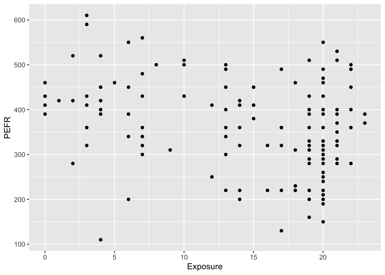
Figure 4-2. Slope and intercept for the regression fit to the lung data
model <- lm(PEFR ~ Exposure, data = lung)
x <- c(7.5, 17.75)
y <- predict(model, newdata = data.frame(Exposure = x))

ggplot(lung, aes(x = Exposure, y = PEFR)) +
  geom_abline(intercept = model$coefficients[1], slope = model$coefficients[2],
    color = "#888888") +
  coord_cartesian(xlim = c(0, 25), ylim = c(300, 450), clip = "off") +
  geom_point(x = 0, y = model$coefficients[1], shape = 3, size = 3) +
  annotate("text", -2.25, model$coefficients[1], label = TeX("$b_0$")) +
  geom_segment(x = x[1], y = y[2], xend = x[2], yend = y[2],
    color = "red", linetype = 3) +
  geom_segment(x = x[1], y = y[1], xend = x[1], yend = y[2],
    color = "red", linetype = 3) +
  annotate("text", x = x[1], y = mean(y), label = TeX("$Delta Y$"),
    hjust = 1.5) +
  annotate("text", x = mean(x), y = y[2], label = TeX("$Delta X$"),
    vjust = 2) +
  annotate("text", x = mean(x), y = 390, label = TeX("$b_1 = \\frac{Delta~Y}{Delta~X}$"))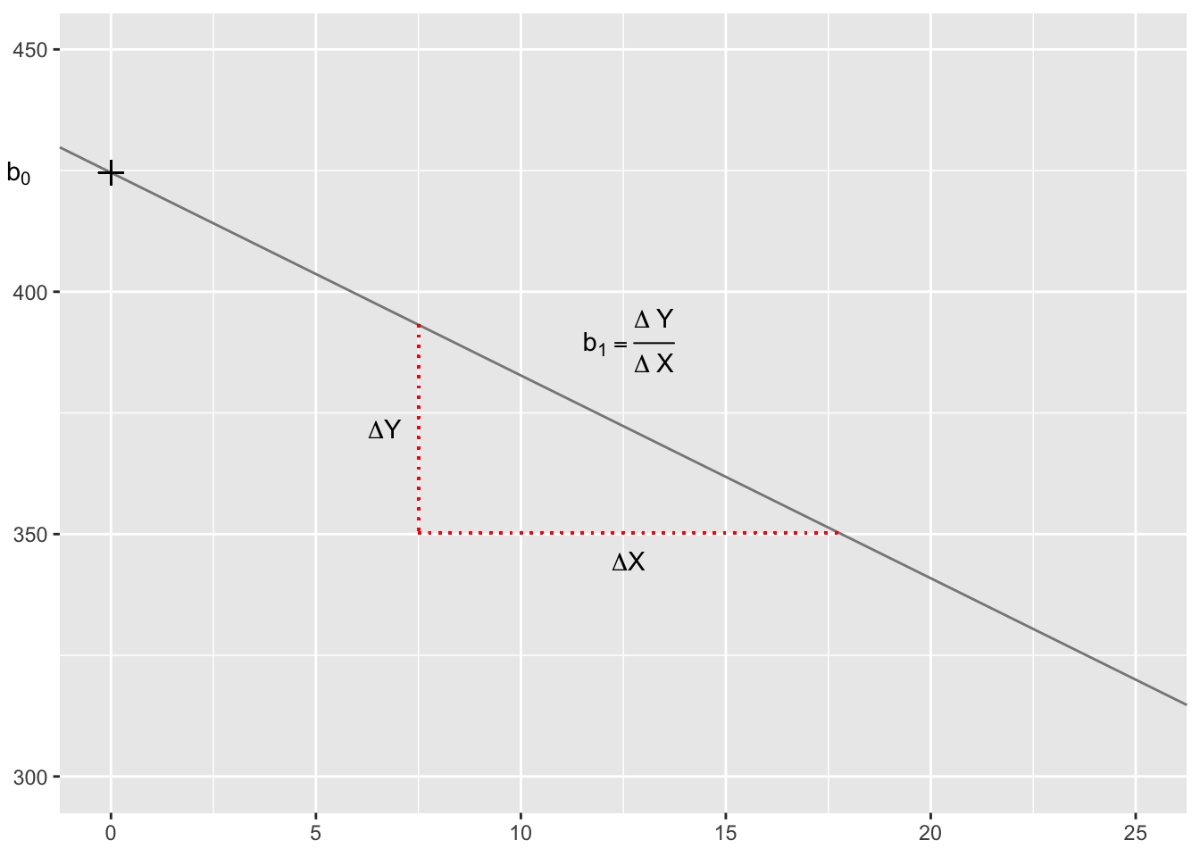
Figure 4-3. Residuals for the regression fit to the lung data
fitted <- predict(model)
resid <- residuals(model)

lung1 <- lung %>%
  mutate(
    Fitted = fitted,
    positive = PEFR > Fitted,
  ) %>%
  group_by(Exposure, positive) %>%
  summarize(
    PEFR_max = max(PEFR),
    PEFR_min = min(PEFR),
    Fitted = first(Fitted),
    .groups = "keep",
  ) %>%
  ungroup() %>%
  mutate(PEFR = ifelse(positive, PEFR_max, PEFR_min)) %>%
  arrange(Exposure)

ggplot(lung1, aes(x = Exposure, y = PEFR, xend = Exposure, yend = Fitted)) +
  geom_abline(intercept = model$coefficients[1], slope = model$coefficients[2],
    color = "grey") +
  geom_segment(linetype = 3, color = "red") +
  geom_point()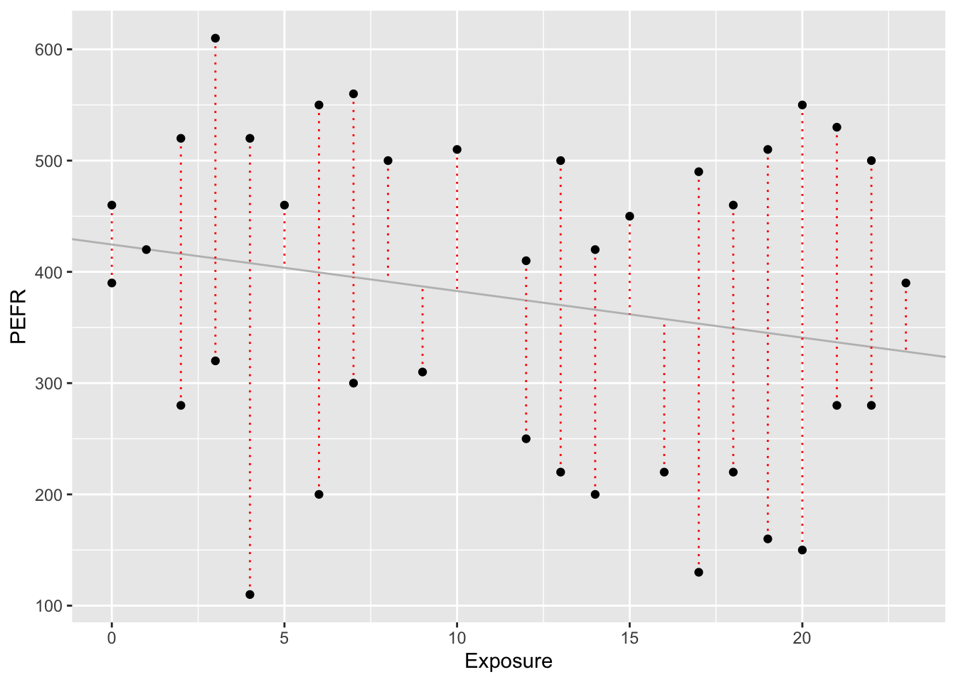
Figure 4-5. An example of an influential data point in regression
seed <- 11
set.seed(seed)

df <- tibble(
  x = rnorm(25),
  y = - x / 5 + rnorm(25)
)
df$x[1] <- 8
df$y[1] <- 8

model1 <- lm(y ~ x, data = df)
model2 <- lm(y[-1] ~ x[-1], data = df)

g <- ggplot(df, aes(x = x, y = y)) +
  geom_point() +
  coord_cartesian(xlim = c(-2.5, 8.5), ylim = c(-2.5, 8.5)) +
  geom_abline(intercept = model1$coefficients[1], slope = model1$coefficients[2],
    col = "blue") +
  geom_abline(intercept = model2$coefficients[1], slope = model2$coefficients[2],
    col = "red", linetype = 2)
g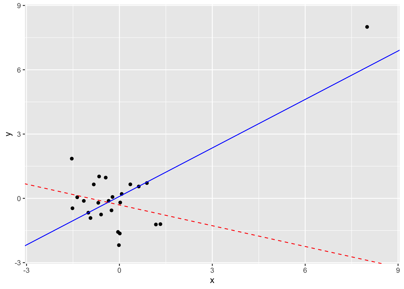
Figure 4-8. A histogram of the residuals from the regression of the housing data
ggplot(tibble(x = df_influential$std_resid), aes(x = x)) +
  geom_histogram(bins = 14) +
  labs(x = "std. residual", y = "Frequency")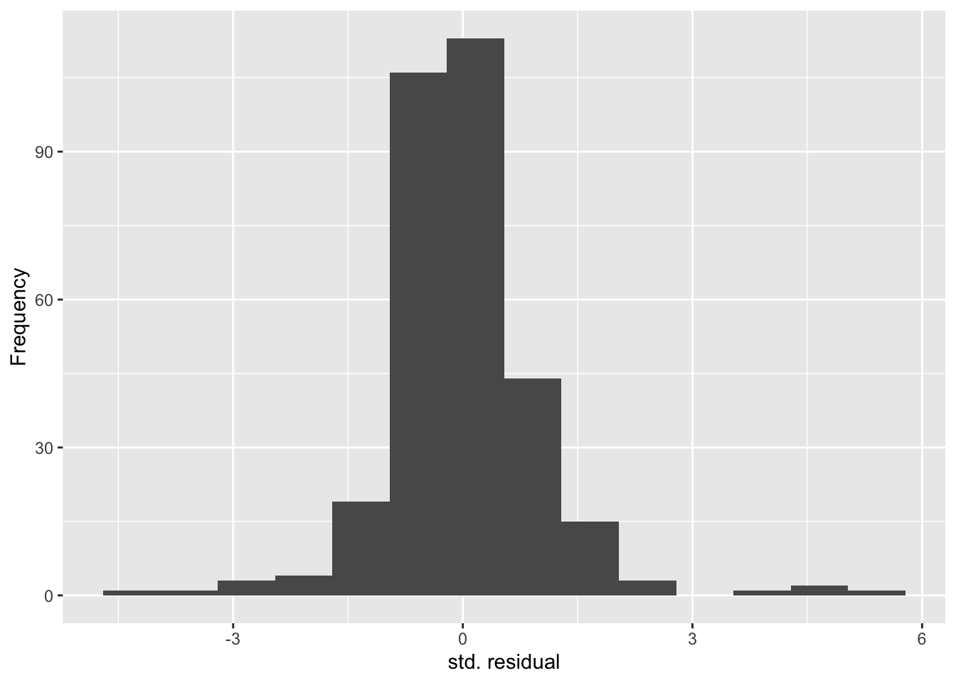
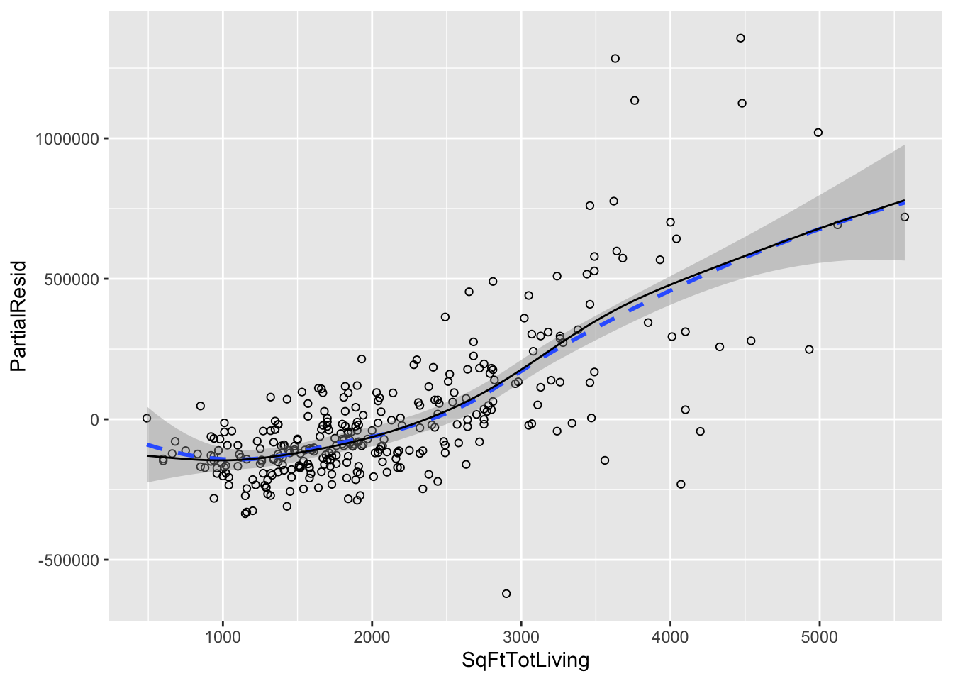
Figure 4-10. A polynomial regression fit for the variable SqFtTotLiving
(solid line) versus a smooth (dashed line; see the following section about splines)
terms <- predict(lm_poly, type = "terms")
partial_resid <- resid(lm_poly) + terms
df <- data.frame(SqFtTotLiving = house_98105[, "SqFtTotLiving"],
  Terms = terms[, 1],
  PartialResid = partial_resid[, 1])
graph <- ggplot(df, aes(SqFtTotLiving, PartialResid)) +
  geom_point(shape = 1) +
  scale_shape(solid = FALSE) +
  geom_smooth(linetype = 2, formula = y ~ x, method = "loess") +
  geom_line(aes(SqFtTotLiving, Terms)) +
  scale_y_continuous(labels = function(x) format(x, scientific = FALSE))
graph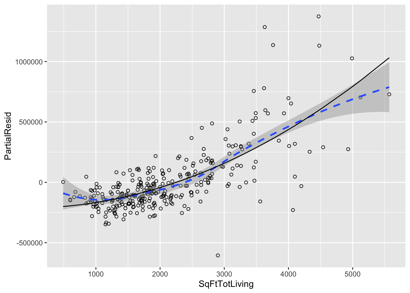
Figure 4-12. A spline regression fit for the variable SqFtTotLiving (solid line) compared to a smooth (dashed line)
terms1 <- predict(lm_spline, type = "terms")
partial_resid1 <- resid(lm_spline) + terms1
df1 <- data.frame(SqFtTotLiving = house_98105[, "SqFtTotLiving"],
  Terms = terms1[, 1],
  PartialResid = partial_resid1[, 1])

graph <- ggplot(df1, aes(SqFtTotLiving, PartialResid)) +
  geom_point(shape = 1) +
  scale_shape(solid = FALSE) +
  geom_smooth(linetype = 2, formula = y ~ x, method = "loess") +
  geom_line(aes(SqFtTotLiving, Terms)) +
  scale_y_continuous(labels = function(x) format(x, scientific = FALSE))
graph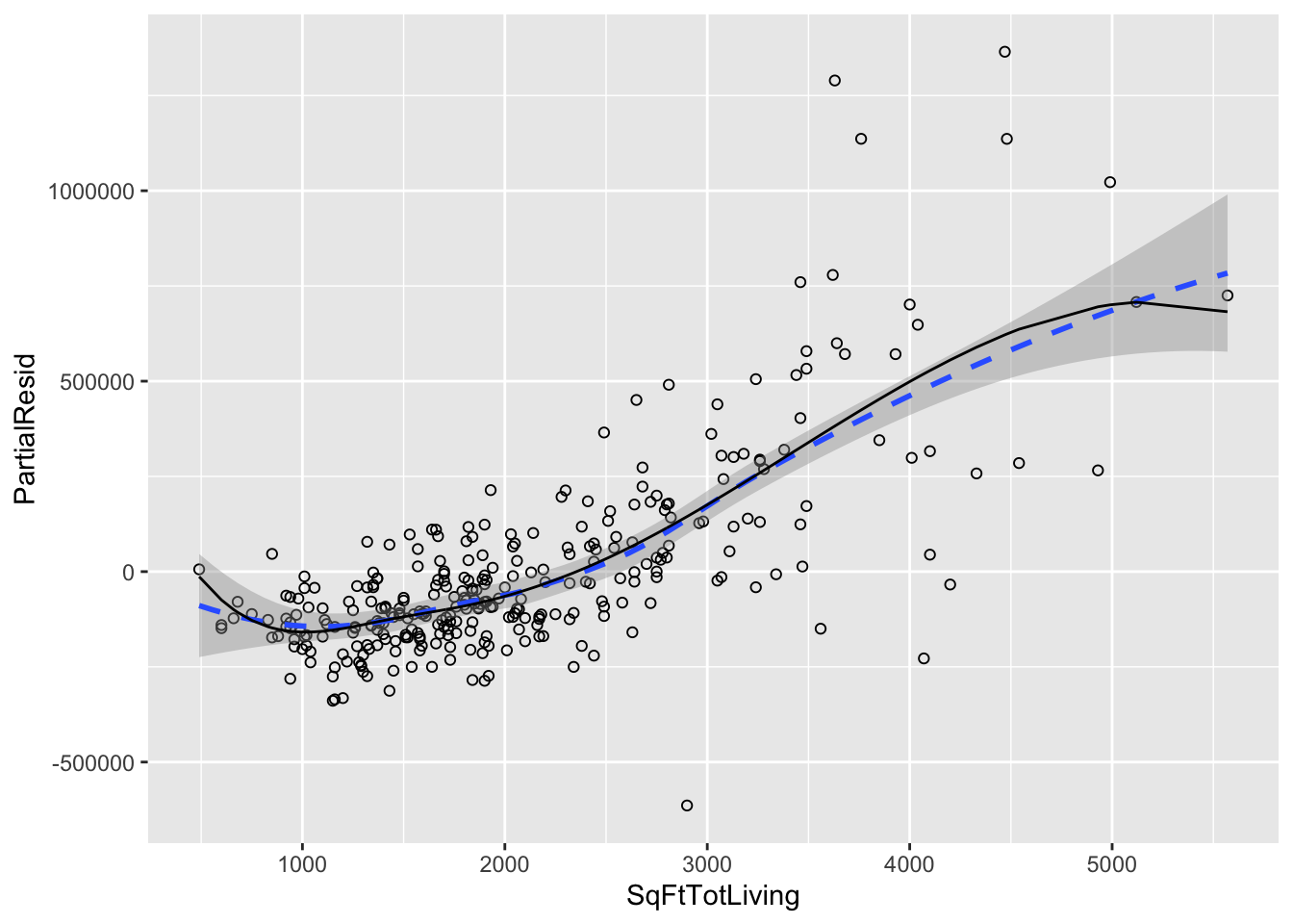
Figure 4-13. A GAM regression fit for the variable SqFtTotLiving (solid line) compared to a smooth (dashed line)
terms <- predict.gam(lm_gam, type = "terms")
partial_resid <- resid(lm_gam) + terms
df <- data.frame(SqFtTotLiving = house_98105[, "SqFtTotLiving"],
  Terms = terms[, 5],
  PartialResid = partial_resid[, 5])
graph <- ggplot(df, aes(SqFtTotLiving, PartialResid)) +
  geom_point(shape = 1) +
  scale_shape(solid = FALSE) +
  geom_smooth(linetype = 2, formula = y ~ x, method = "loess") +
  geom_line(aes(SqFtTotLiving, Terms)) +
  scale_y_continuous(labels = function(x) format(x, scientific = FALSE))
graph