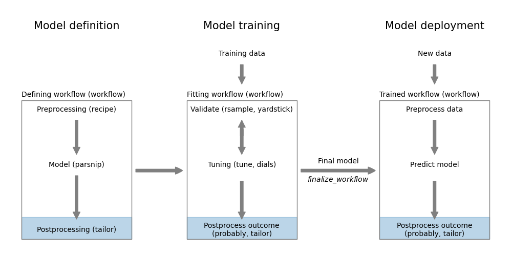
8 Postprocessing model predictions

It’s not always possible to directly use the raw outputs of a model to make a decision. We may need to apply some postprocessing steps to convert the raw outputs into a more usable form.

8.1 Why postprocess model predictions?

Before we look into specific ways of postprocessing model predictions in tidymodels, let’s first see why postprocessing may be necessary.

8.1.1 Classification

Most classification models output scores or probabilities that need to be converted into class labels. This conversion is done by applying a threshold. The default threshold is usually 0.5, but this can be adjusted based on the specific requirements of the problem. For example, if we want to minimize false negatives, we may want to lower the threshold to increase sensitivity. On the other hand, if we want to minimize false positives, we may want to raise the threshold to increase specificity.

Threshold selection doesn’t require the model output to be a probability. However, if we are interested in probabilities and the model outputs scores, we can use a calibration method to convert the scores into probabilities. Calibration methods include Platt scaling and isotonic regression. These methods align the predicted probabilities with the true likelihoods of the classes.

8.1.2 Regression

Sometimes, we need to transform the outcome of a regression model before it can be used in training. This could be a log-transformation or a Box-Cox transformation to make the data more normally distributed. It could also be just a form of linear scaling to make the training more stable. In these cases, we need to apply the inverse transformation to the predictions of the model to get them back into the original scale.

There can also be cases where we need to calibrate the outcome using a non-linear, isotonic transformation. Isotonic means that the transformation is monotone increasing. This can be useful when the model is systematically underestimating or overestimating the true values as is often the case at the edges of the distribution. By applying an isotonic transformation, we can adjust the predictions to better match the true values.

8.2 Postprocessing in classification

The tidymodels framework provides two packages that deal with postprocessing: probably and tailor.

Postprocessing using probably — Figure 8.1: Postprocessing using `probably`

In this chapter, we will see examples of using both packages. The probably package is designed for postprocessing classification model predictions. While it works well with tidymodels, it is not as well integrated as the tailor package. This package implements functionality for both regression and classification. It is however newer and still under development.

We first load the necessary packages.

library(tidyverse)
library(tidymodels)
library(yardstick)
library(probably)  # for exploring thresholds
library(tailor)   # for including postprocessing in workflows
library(patchwork) # for combining plots
library(ranger)

Then we define classification models.

file <- paste0(
  "https://gedeck.github.io/machine-learning-with-tidymodels/",
  "datasets/UniversalBank.csv.gz"
)
data <- read_csv(file)
data <- data |>
  select(-c(ID, `ZIP Code`)) |>
  rename(
    Personal.Loan = `Personal Loan`,
    Securities.Account = `Securities Account`,
    CD.Account = `CD Account`
  ) |>
  mutate(
    Personal.Loan = factor(Personal.Loan, labels = c("Yes", "No"),
      levels = c(1, 0)),
    Education = factor(Education,
      labels =  c("Undergrad", "Graduate", "Advanced")),
  )
formula <- Personal.Loan ~ Income + Family + CCAvg + Education +
  Mortgage + Securities.Account + CD.Account + Online + CreditCard
rec <- recipe(formula, data = data)
classification_wf <- workflow() |>
  add_recipe(rec) |>
  add_model(logistic_reg())
classification_model <- fit(classification_wf, data = data)

8.2.1 Threshold selection using `probably`

Selecting the best threshold is a trade-off between sensitivity and specificity. The probably package provides a function to explore the relationship between thresholds and performance metrics. The function probably::threshold_perf calculates the performance metrics for a range of thresholds. The function returns a tibble with the threshold, the performance metric, and the estimate. We can use this tibble to plot the relationship between thresholds and performance metrics and determine a threshold based on a criteria of our choice. Figure 8.2 shows the relationship between thresholds and accuracy, sensitivity, and specificity.

pred_data <- augment(classification_model, new_data = data)
performance_1 <- probably::threshold_perf(pred_data, Personal.Loan,
  .pred_Yes, thresholds = seq(0.05, 0.95, 0.01),
  event_level = "first",
  metrics = metric_set(j_index, specificity, sensitivity))
performance_2 <- probably::threshold_perf(pred_data, Personal.Loan,
  .pred_Yes, thresholds = seq(0.05, 0.95, 0.01),
  event_level = "first",
  metrics = metric_set(accuracy, kap, bal_accuracy, f_meas))
max_j_index <- performance_1 |>
  filter(.metric == "j_index") |>
  filter(.estimate == max(.estimate))
max_performance <- performance_2 |>
  arrange(desc(.threshold)) |>
  group_by(.metric) |>
  filter(.estimate == max(.estimate)) |>
  filter(row_number() == 1)

g1 <- ggplot(performance_1,
  aes(x = .threshold, y = .estimate, color = .metric,
    linetype = .metric)) +
  geom_line() +
  geom_vline(data = max_j_index,
    aes(xintercept = .threshold, color = .metric)) +
  scale_x_continuous(breaks = seq(0, 1, 0.1)) +
  xlab("Threshold") + ylab("Metric value") +
  theme(legend.position = "inside",
    legend.position.inside = c(0.85, 0.75))
g2 <- ggplot(performance_2,
  aes(x = .threshold, y = .estimate, color = .metric,
    linetype = .metric)) +
  geom_line() +
  geom_vline(data = max_performance,
    aes(xintercept = .threshold, color = .metric)) +
  scale_x_continuous(breaks =  seq(0, 1, 0.1)) +
  xlab("Threshold") + ylab("Metric value") +
  theme(legend.position = "inside",
    legend.position.inside = c(0.85, 0.75))
g1 + g2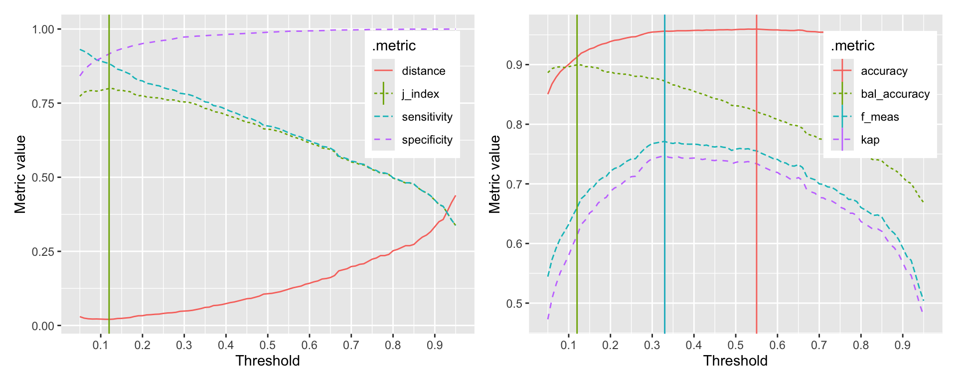

Figure 8.2: Relationship between threshold and sensitivity, specificity, and j-index

The probably::threshold_perf function takes a tibble and the names of the columns that contain the truth and the predicted probabilities. The thresholds argument specifies the range of thresholds to be explored. The metrics argument specifies the metrics to be calculated for each threshold. If your event of interest is not the first level, you can specify this using the event_level argument. Evaluating the performance metrics is very fast, so you can explore a large number of thresholds. Here, we explored 91 thresholds between 0.05 and 0.95.

The graphs clearly show that depending on the selected metric, the optimal threshold is different. The first graph shows the relationship between thresholds and the J-index, sensitivity, and specificity. The second graph shows the relationship between thresholds and accuracy, kappa, and balanced accuracy. The vertical lines indicate the optimal threshold for each metric. The optimal threshold for the J-index is 0.12. The optimal thresholds for accuracy, kappa, F-measure, and balanced accuracy are 0.55, 0.33, 0.33, 0.12 respectively.

8.2.2 Incorporating postprocessing into workflows

To incorporate postprocessing into a workflow, we use the add_tailor function. Here is an example, where we adjust the threshold of a classification model to 0.1.

adj_tailor <- tailor() |>
  adjust_probability_threshold(threshold = 0.1)

adj_classification_wf <- workflow() |>
  add_recipe(rec) |>
  add_model(logistic_reg()) |>
  add_tailor(adj_tailor)
adj_classification_model <- fit(adj_classification_wf, data = data)

With the different threshold, the confusion matrix changes as we can see in the output below.

augment(classification_model, new_data = data) |>
  accuracy(truth = Personal.Loan, estimate = .pred_class)

# A tibble: 1 × 3
  .metric  .estimator .estimate
  <chr>    <chr>          <dbl>
1 accuracy binary         0.959

augment(adj_classification_model, new_data = data) |>
  accuracy(truth = Personal.Loan, estimate = .pred_class)

# A tibble: 1 × 3
  .metric  .estimator .estimate
  <chr>    <chr>          <dbl>
1 accuracy binary         0.900

With the adjusted threshold, the accuracy of the original model drops to around 0.9. This is what we would expect from Figure 8.2.

8.2.3 Threshold tuning as part of the workflow

In this example, we adjusted the threshold using a fixed value. In the same way that we tune preprocessing and model parameters, we can also tune the threshold. Without going into the details of tuning itself (see Chapter 15 and Chapter 16) the following code demonstrates threshold tuning.

set.seed(123)
folds <- vfold_cv(data, v = 10, strata = Personal.Loan)
1cv_metrics <- metric_set(f_meas)

tune_tailor <- tailor() |>
2  adjust_probability_threshold(threshold = tune())
tune_wf <- workflow() |>
  add_recipe(rec) |>
  add_model(logistic_reg()) |>
  add_tailor(tune_tailor)

parameters <- extract_parameter_set_dials(tune_wf) |>
3  update(threshold = threshold(range = c(0.1, 0.9)))

threshold_tune <- tune_bayes(tune_wf, resamples = folds,
  metrics = cv_metrics,
  param_info = parameters, iter = 25)

1: We use the F-measure as the metric to optimize in tuning
2: We mark the threshold as a tunable parameter using the tune() function
3: We specify the range to avoid getting extreme threshold values that are not useful in practice.

! No improvement for 10 iterations; returning current results.

autoplot(threshold_tune)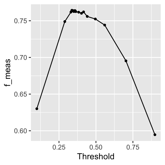

Figure 8.3: Tune threshold as part of the workflow

The autoplot in Figure 8.3 shows the result of the tuning. The relationship is similar to what we’ve seen in Figure 8.2.

best_threshold <- threshold_tune |>
  select_best(metric = "f_meas")
best_threshold

# A tibble: 1 × 2
  threshold .config
      <dbl> <chr>  
1     0.337 iter08

The optimal threshold is similar to what we found in Figure 8.2.

Useful to know

This section has shown you how to calculate classification metrics as a function of the threshold. In any project, you will need to decide which of all possible metrics is the most appropriate for your problem. Sometimes you want to be more risk averse and prefer a higher sensitivity or fewer false negatives. Sometimes you can be more risk taking and prefer a higher specificity or fewer false positives.

8.3 Postprocessing in regression

Postprocessing can be done using tailor. For this section, we use a random forest model that we train and validate using cross-validation.

data <- ISLR2::Carseats
formula <- Sales ~ .
set.seed(1234)
folds <- vfold_cv(data, strata = Sales)

regression_wf <- workflow() |>
  add_recipe(recipe(formula, data = data)) |>
  add_model(rand_forest(mode = "regression", trees = 1000))
res_cv <- fit_resamples(regression_wf, resamples = folds,
  control = control_resamples(save_pred = TRUE))

The calibration plot in Figure 8.4 shows that the model is systematically overestimating the true values for low sales and underestimating them for high sales. The adjust_numeric_calibration function can reduce this problem.

calibrated_wf <- regression_wf |>
  add_tailor(tailor() |>
1      adjust_numeric_calibration())
calibrated_cv <- fit_resamples(calibrated_wf, resamples = folds,
  control = control_resamples(save_pred = TRUE))

1: We add the adjust_numeric_calibration function to the workflow using add_tailor.

The adjust_numeric_calibration function fits a generalized additive model. Figure 8.4 shows the regression calibration plot for the original and the calibrated model. The calibrated model improves the under- and overestimation of the original model.

g1 <- collect_predictions(res_cv) |>
  cal_plot_regression(truth = Sales, estimate = .pred) +
  ggtitle("Uncalibrated model")
g2 <- collect_predictions(calibrated_cv) |>
  cal_plot_regression(truth = Sales, estimate = .pred) +
  ggtitle("Calibrated model")
g1 + g2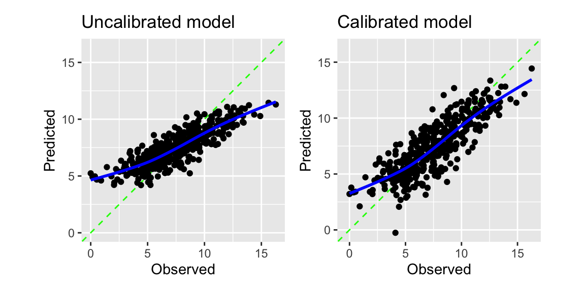

There is nothing like a free lunch in machine learning. We can see this from the performance metrics of the original and the calibrated model. The calibration improved the regression calibration plot and the RMSE, but at the same time, the R-squared was reduced slightly.

bind_rows(
  collect_metrics(res_cv) |> mutate(model = "Uncalibrated"),
  collect_metrics(calibrated_cv) |> mutate(model = "Calibrated")
) |>
  select(model, .metric, mean) |>
  pivot_wider(names_from = .metric, values_from = mean) |>
  knitr::kable(digits = 3) |>
  kableExtra::kable_styling(full_width = FALSE)

model	rmse	rsq
Uncalibrated	1.683	0.728
Calibrated	1.590	0.704

Further information

The tidymodels packages probably and tailor are the packages covered in this section. You find more details about these packages in the following links:

https://probably.tidymodels.org/ is the documentation for the probably package.
https://tailor.tidymodels.org/reference/index.html is the documentation for the tailor package.
This Blogpost from 2024 introduces the tailor package.
More on calibration

Code

The code of this chapter is summarized here.

Show the code

knitr::opts_chunk$set(echo = TRUE, cache = TRUE, autodep = TRUE,
  fig.align = "center")
knitr::include_graphics("images/model_workflow_tailor.png")
library(tidyverse)
library(tidymodels)
library(yardstick)
library(probably)  # for exploring thresholds
library(tailor)   # for including postprocessing in workflows
library(patchwork) # for combining plots
library(ranger)
file <- paste0(
  "https://gedeck.github.io/machine-learning-with-tidymodels/",
  "datasets/UniversalBank.csv.gz"
)
data <- read_csv(file)
data <- data |>
  select(-c(ID, `ZIP Code`)) |>
  rename(
    Personal.Loan = `Personal Loan`,
    Securities.Account = `Securities Account`,
    CD.Account = `CD Account`
  ) |>
  mutate(
    Personal.Loan = factor(Personal.Loan, labels = c("Yes", "No"),
      levels = c(1, 0)),
    Education = factor(Education,
      labels =  c("Undergrad", "Graduate", "Advanced")),
  )
formula <- Personal.Loan ~ Income + Family + CCAvg + Education +
  Mortgage + Securities.Account + CD.Account + Online + CreditCard
rec <- recipe(formula, data = data)
classification_wf <- workflow() |>
  add_recipe(rec) |>
  add_model(logistic_reg())
classification_model <- fit(classification_wf, data = data)
pred_data <- augment(classification_model, new_data = data)
performance_1 <- probably::threshold_perf(pred_data, Personal.Loan,
  .pred_Yes, thresholds = seq(0.05, 0.95, 0.01),
  event_level = "first",
  metrics = metric_set(j_index, specificity, sensitivity))
performance_2 <- probably::threshold_perf(pred_data, Personal.Loan,
  .pred_Yes, thresholds = seq(0.05, 0.95, 0.01),
  event_level = "first",
  metrics = metric_set(accuracy, kap, bal_accuracy, f_meas))
max_j_index <- performance_1 |>
  filter(.metric == "j_index") |>
  filter(.estimate == max(.estimate))
max_performance <- performance_2 |>
  arrange(desc(.threshold)) |>
  group_by(.metric) |>
  filter(.estimate == max(.estimate)) |>
  filter(row_number() == 1)

g1 <- ggplot(performance_1,
  aes(x = .threshold, y = .estimate, color = .metric,
    linetype = .metric)) +
  geom_line() +
  geom_vline(data = max_j_index,
    aes(xintercept = .threshold, color = .metric)) +
  scale_x_continuous(breaks = seq(0, 1, 0.1)) +
  xlab("Threshold") + ylab("Metric value") +
  theme(legend.position = "inside",
    legend.position.inside = c(0.85, 0.75))
g2 <- ggplot(performance_2,
  aes(x = .threshold, y = .estimate, color = .metric,
    linetype = .metric)) +
  geom_line() +
  geom_vline(data = max_performance,
    aes(xintercept = .threshold, color = .metric)) +
  scale_x_continuous(breaks =  seq(0, 1, 0.1)) +
  xlab("Threshold") + ylab("Metric value") +
  theme(legend.position = "inside",
    legend.position.inside = c(0.85, 0.75))
g1 + g2
adj_tailor <- tailor() |>
  adjust_probability_threshold(threshold = 0.1)

adj_classification_wf <- workflow() |>
  add_recipe(rec) |>
  add_model(logistic_reg()) |>
  add_tailor(adj_tailor)
adj_classification_model <- fit(adj_classification_wf, data = data)
augment(classification_model, new_data = data) |>
  accuracy(truth = Personal.Loan, estimate = .pred_class)
augment(adj_classification_model, new_data = data) |>
  accuracy(truth = Personal.Loan, estimate = .pred_class)
set.seed(123)
folds <- vfold_cv(data, v = 10, strata = Personal.Loan)
cv_metrics <- metric_set(f_meas)

tune_tailor <- tailor() |>
  adjust_probability_threshold(threshold = tune())
tune_wf <- workflow() |>
  add_recipe(rec) |>
  add_model(logistic_reg()) |>
  add_tailor(tune_tailor)

parameters <- extract_parameter_set_dials(tune_wf) |>
  update(threshold = threshold(range = c(0.1, 0.9)))

threshold_tune <- tune_bayes(tune_wf, resamples = folds,
  metrics = cv_metrics,
  param_info = parameters, iter = 25)
autoplot(threshold_tune)
best_threshold <- threshold_tune |>
  select_best(metric = "f_meas")
best_threshold
data <- ISLR2::Carseats
formula <- Sales ~ .
set.seed(1234)
folds <- vfold_cv(data, strata = Sales)

regression_wf <- workflow() |>
  add_recipe(recipe(formula, data = data)) |>
  add_model(rand_forest(mode = "regression", trees = 1000))
res_cv <- fit_resamples(regression_wf, resamples = folds,
  control = control_resamples(save_pred = TRUE))
calibrated_wf <- regression_wf |>
  add_tailor(tailor() |>
      adjust_numeric_calibration())
calibrated_cv <- fit_resamples(calibrated_wf, resamples = folds,
  control = control_resamples(save_pred = TRUE))
g1 <- collect_predictions(res_cv) |>
  cal_plot_regression(truth = Sales, estimate = .pred) +
  ggtitle("Uncalibrated model")
g2 <- collect_predictions(calibrated_cv) |>
  cal_plot_regression(truth = Sales, estimate = .pred) +
  ggtitle("Calibrated model")
g1 + g2
bind_rows(
  collect_metrics(res_cv) |> mutate(model = "Uncalibrated"),
  collect_metrics(calibrated_cv) |> mutate(model = "Calibrated")
) |>
  select(model, .metric, mean) |>
  pivot_wider(names_from = .metric, values_from = mean) |>
  knitr::kable(digits = 3) |>
  kableExtra::kable_styling(full_width = FALSE)