Off-Line Quality Control, Parameter Design and The Taguchi Method

The performance of products or processes is typically quantified by performance measures. Examples include measures such as piston cycle time, yield of a production process, output voltage of an electronic circuit, noise level of a compressor or response times of a computer system. These performance measures might be affected by several factors that have to be set at specific levels to get desired results. For example the piston simulator introduced in previous chapters has seven factors that can be used to control the piston cycle time. The aim of off-line quality control is to determine the factor-level combination that gives the least variability to the appropriate performance measure, while keeping the mean value of the measure on target. The goal is to control both accuracy and variability. In the next section we discuss an optimization strategy that solves this problem by minimizing various loss functions.

Product and Process Optimization using Loss Functions

Optimization problems of products or processes can take many forms that depend on the objectives to be reached. These objectives are typically derived from customer requirements. Performance parameters such as dimensions, pressure or velocity usually have a target or nominal value. The objective is to reach the target within a range bounded by upper and lower specification limits. We call such cases nominal is best. Noise levels, shrinkage factors, amount of wear and deterioration are usually required to be as low as possible. We call such cases the smaller the better. When we measure strength, efficiency, yields or time to failure our goal is, in most cases, to reach the maximum possible levels. Such cases are called the larger the better. These three types of cases require different objective (target) functions to optimize. Taguchi introduced the concept of loss function to help determine the appropriate optimization procedure.

When nominal is best specification limits are typically two sided with an upper specification limit (USL) and a lower specification limit (LSL). These limits are used to differentiate between conforming and nonconforming products. Nonconforming products are usually fixed, retested and sometimes downgraded or simply scrapped. In all cases defective products carry a loss to the manufacturer. Taguchi argues that only products on target should carry no loss. Any deviation carries a loss which is not always immediately perceived by the customer or production personnel. Taguchi proposes a quadratic function as a simple approximation to a graduated loss function that measures loss on a continuous scale. A quadratic loss function has the form

$L(y,M) = K(y-M)^2,$

where $y$ is the value of the performance characteristic of a product, $M$ is the target value of this characteristic and $K$ is a positive constant, which yields monetary or other utility value to the loss. For example, suppose that $(M-\Delta,M+\Delta)$ is the customer’s tolerance interval around the target. When $y$ falls out of this interval the product has to be repaired or replaced at a cost of $ $A$. Then, for this product,

$A = K\Delta^2$

or

$K = A/\Delta^2.$

The manufacturer’s tolerance interval is generally tighter than that of the customer, namely $(M-\delta,M+\delta)$, where $\delta < \Delta$. One can obtain the value of $\delta$ in the following manner. Suppose the cost to the manufacturer to repair a product that exceeds the customer’s tolerance, before shipping the product, is $ $B$, $B < A$. Then

$B = \left(\frac{A}{\Delta^2}\right) (Y-M)^2,$

or

$Y = M \pm \Delta\left(\frac{B}{A}\right)^{1/2}.$

Thus,

$\delta = \Delta\left(\frac{B}{A}\right)^{1/2}.$

The manufacturer should reduce the variability in the product performance characteristic so that process capability $C_{pk}$ for the tolerance interval $(M-\delta,M+\delta)$ should be high. See Fig. 6.1 for a schematic presentation of these relationships.

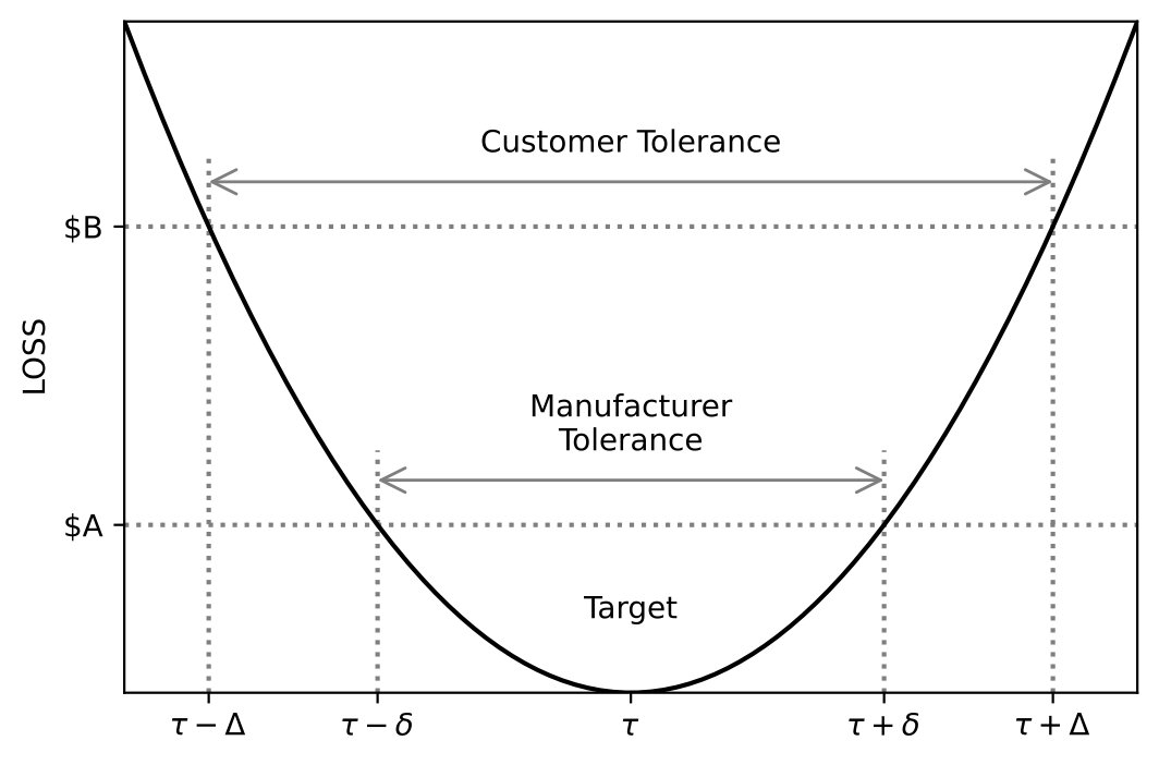
Fig. 6.1 Quadratic Loss and Tolerance Intervals

Notice that the expected loss is

$E{L(Y,M)} = K(\text{Bias}^2 + \text{Variance})$

where Bias $= \mu - M$, $\mu = E{Y}$ and Variance $= E{(Y-\mu)^2}$. Thus, the objective is to have a manufacturing process with $\mu$ as close as possible to the target $M$, and variance, $\sigma^2$, as small as possible $(\sigma < \frac{\delta}{3}$ so that $C_{pk} > 1$). Recall that Variance + Bias $^2$ is the Mean Squared Error, MSE. Thus, when normal is best the objective should be to minimize the MSE.

Objective functions for cases of the bigger the better or the smaller the better depend on the case under consideration. In cases where the performance measure is the life length of a product, the objective might be to design the product to maximize the expected life length. In the literature we may find the objective of minimizing $\frac{1}{n} \sum \frac{1}{y^j}$, which is an estimator of $E(\frac{1}{Y})$. This parameter, however, may not always exist (e.g. when $Y$ has an exponential distribution), and this objective function might be senseless.